ML Interview Q Series: In anomaly detection, how would you describe the issues known as Swamping and Masking, and why do they occur?

📚 Browse the full ML Interview series here.

Comprehensive Explanation

Understanding Anomaly Detection Anomaly Detection refers to the task of identifying unusual patterns or points in data that deviate significantly from the overall majority. Such unusual points are referred to as anomalies, outliers, or aberrations. Various strategies, such as distance-based, density-based, or statistical methods, can be employed. Problems arise when multiple anomalies exist in the data and influence each other’s detection. Two well-known issues in these situations are Swamping and Masking.

Masking Phenomenon Masking occurs when multiple anomalous points blend together in such a way that they appear normal when considered collectively. Because anomalies exert influence on estimated parameters (like the mean or covariance in statistical methods), a large group of outliers can cause the parameter estimates to shift. The outliers then look as if they fit the distribution, and the algorithm fails to flag them as anomalies.

Swamping Phenomenon Swamping is the opposite scenario. When there are multiple anomalies, their presence can distort the parameter estimation so severely that some normal points begin to appear anomalous. The normal points get “swamped” and are falsely flagged because the distribution metrics shift excessively in response to the outliers.

Why Swamping and Masking Occur These issues typically arise in situations where the detection algorithm is sensitive to the overall distribution of data. For instance, in statistical methods that estimate the mean, variance, or covariance of the data distribution, a small group of outliers might skew those estimates significantly, leading to misclassification of both normal points and the outliers themselves.

Illustrating a Typical Distance-Based Criterion A common method for anomaly detection uses distance from a central location measure (for example, the mean vector). One such measure is the Mahalanobis distance, which accounts for correlations among features:

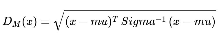
Here, x is the data point in a high-dimensional space, mu is the estimated mean vector of the distribution, and Sigma^{-1} is the inverse of the covariance matrix. When multiple outliers skew mu and Sigma, some normal points become large-distance points (swamping), while some outliers are pulled into a region that looks normal (masking).

Techniques to Mitigate Swamping and Masking Approaches to reduce these issues include using robust statistics that limit the influence of extreme values, or iterative anomaly detection methods that progressively refine estimates. Methods such as M-estimators, median-based estimators, or robust covariance estimation (e.g., Minimum Covariance Determinant) attempt to down-weight the effect of outliers so that parameter estimates remain stable. Density-based methods like DBSCAN also attempt to cluster normal data and separate those clusters from anomalies, potentially reducing the risk of swamping and masking.

Implementation Example in Python Below is a code snippet demonstrating how one might use scikit-learn’s robust covariance for anomaly detection. This approach tries to reduce the effects of outliers on the covariance estimate:

import numpy as np
from sklearn.covariance import EllipticEnvelope

# Generate synthetic data (normal cluster + outliers)
rng = np.random.RandomState(42)
normal_data = 0.5 * rng.randn(100, 2)
outlier_data = rng.uniform(low=-6, high=6, size=(20, 2))
X = np.concatenate([normal_data, outlier_data], axis=0)

# Fit a robust covariance-based anomaly detector
elliptic_env = EllipticEnvelope(contamination=0.2, random_state=42)
elliptic_env.fit(X)

# Predict anomalies
preds = elliptic_env.predict(X)
anomalies = X[preds == -1]
print("Total anomalies detected:", len(anomalies))

By using a robust estimator like EllipticEnvelope with a contamination parameter set to a certain fraction of outliers, the impact of multiple anomalies can be limited, thereby reducing the chances of swamping and masking.

Follow-Up Questions

Could you explain how robust statistical estimators help mitigate Swamping and Masking?

Robust statistical estimators reduce the impact that extreme points have on the estimation of parameters such as location and scale. Many classical estimators (like the sample mean and covariance) place equal weight on all observations. This can cause parameter estimates to shift drastically when multiple outliers are present. Robust estimators, on the other hand, intentionally ignore or down-weight extreme points, preventing them from distorting the estimates for normal data. Techniques such as M-estimators or median-based methods are designed with bounded influence functions that ensure a large cluster of outliers does not dominate the parameter estimates.

How do methods based on local density (for instance, Local Outlier Factor) deal with these issues?

Local density methods identify anomalies by comparing each point’s neighborhood density to the density of its neighbors. Even if many outliers exist, those anomalies typically have a lower density compared to normal clusters, and their local neighborhoods reflect that. This approach can partially circumvent the problem of swamping and masking because it does not rely on a single global parameter estimate. Instead, it derives an anomaly score by looking at differences in local data structure. However, if outliers form dense subgroups, there is still some potential for masking if that subgroup is dense relative to its immediate vicinity.

In real-world scenarios with high-dimensional data, how do we detect and address Swamping and Masking?

In high-dimensional settings, distance and density measures can become unreliable due to the curse of dimensionality, making swamping and masking more frequent. Techniques such as dimensionality reduction (PCA, t-SNE, autoencoders) can help by mapping data to a lower-dimensional space where the structure is more discernible. Robust versions of these techniques or methods specifically designed for high-dimensional anomaly detection (like isolation forests or subspace-based clustering) also help. Isolation Forest, for example, isolates points by randomly splitting feature dimensions, making it less dependent on a strict global distribution estimate and reducing the severity of swamping and masking.

How does one diagnose whether the model is experiencing Masking or Swamping?

One way is to examine diagnostic plots, such as plotting the residual errors or the Mahalanobis distances, and seeing whether certain clusters appear to have a suspiciously uniform distance distribution. Another strategy is to remove a small subset of points identified as potential anomalies and rerun the model to see if many more points suddenly become flagged as outliers (which could indicate that original outliers were masking others). Likewise, if removing suspected outliers results in fewer points being flagged, it could mean that swamping was occurring.

Is it possible that unsupervised anomaly detection approaches fail if a large group of anomalies dominate the data?

Yes, unsupervised approaches without labeled data rely purely on patterns inherent in the dataset. If the fraction of anomalies is significant, the algorithm’s underlying assumptions might be violated. For instance, robust covariance-based estimators still assume that the majority of data is normal. If outliers constitute a substantial share, the estimators could adapt more to outliers than normal data, leading to mask or swamp effects. It’s often necessary to have some domain knowledge, or at least an approximate idea of the anomaly rate, to set hyperparameters (like contamination) in ways that mitigate these issues.

Below are additional follow-up questions

In real-world applications, how do you handle situations where anomalies are not errors but carry important information?

Many industries (healthcare, finance, cybersecurity) view anomalous points as potential indicators of critical events. If these anomalies are genuinely informative rather than mistakes, the data scientist must adjust the approach:

One important step is collecting domain knowledge to differentiate between “noise” anomalies (errors or artifacts) and “event” anomalies (significant but rare patterns). For example, in healthcare data, sudden spikes in a patient’s vital signs might be false alarms, but they could also be life-saving signals. You might adopt a semi-supervised strategy, where subject matter experts label some instances as meaningful anomalies. This labeled set guides your choice of model or helps you calibrate detection thresholds.

A common pitfall is failing to communicate with domain experts. For example, if a financial institution sees unusual account transactions, purely statistical methods might wrongly group them with trivial noise, while a domain expert can confirm suspicious activities. Another risk is overfitting a model to treat all deviations as anomalies, which might bury genuinely meaningful signals under false positives. Ultimately, you want to incorporate domain-driven thresholds and interpretability measures (like feature importance for each outlier) to accurately catch significant events.

How can domain-specific knowledge help prevent Swamping and Masking in practice?

Domain-specific knowledge often provides context about typical data ranges, correlations among features, or expected anomaly proportions. If you know that a dataset should contain only a small fraction of anomalies, you can fine-tune your model (for example, setting the contamination parameter in robust estimators) to reflect that. In a medical diagnosis scenario, domain experts might know that certain vitals can spike simultaneously without indicating pathology, thus reducing the likelihood of misclassifying normal data as anomalies (swamping). Conversely, experts could flag certain subtle correlations that indicate true anomalies, even if they are visually “clustered” with normal points (masking).

A subtle challenge is when domain knowledge is incomplete or contradictory. Different experts may disagree on what constitutes an anomaly. Additionally, domain knowledge may introduce biases if the known patterns are outdated. For instance, in cybersecurity, new attack vectors may not align with historically recognized patterns. Addressing these pitfalls involves periodically revisiting and updating domain assumptions, and potentially maintaining multiple models that incorporate different expertise sources.

What are the benefits and pitfalls of using ensemble methods to address Swamping and Masking?

Ensemble approaches combine multiple anomaly detection models (for instance, combining a robust covariance method with a density-based method). When these models disagree, it can indicate cases at higher risk of swamping or masking. By aggregating results—through voting or averaging anomaly scores—you reduce reliance on any single parameter estimate that outliers could skew. This typically makes it harder for multiple anomalies to distort the entire detection process in a uniform way.

Pitfalls emerge if the component models in the ensemble are highly correlated or all vulnerable to the same distortions. For example, multiple distance-based methods might still shift their shared parameters similarly when confronted with a large cluster of outliers. Additionally, building and tuning an ensemble can be computationally expensive, especially in large-scale, high-dimensional contexts. Another subtle issue is how to reconcile different scoring scales across diverse models (e.g., a probability from a Gaussian-based method versus a distance measure from a nearest-neighbor approach). Failing to properly scale or weight these scores could lead to misclassification errors.

How do you select a proper threshold or contamination parameter in the absence of labeled anomalies?

In unsupervised anomaly detection, the contamination parameter (or decision threshold) often dictates the expected proportion of outliers. Without labeled data, you might use a combination of unsupervised strategies. One practical technique is the “elbow method,” where you look at the distribution of anomaly scores or distances and search for a sharp inflection point. Another is to carry out domain-driven stress tests: artificially inject a few synthetic outliers into your dataset and adjust thresholds until those injected anomalies are consistently detected. Monitoring performance on these synthetic outliers can guide parameter selection.

However, synthetic insertion can fail if it does not accurately resemble real anomalies—especially if the real anomalies are more subtle or clustered in unusual feature subspaces. Another pitfall is selecting a threshold that works well on a small test sample but fails to generalize. Continual monitoring of your anomaly rates and gathering feedback from real-world usage can help refine the threshold over time.

How should you adapt an anomaly detection system when data distributions shift or evolve over time?

Concept drift or distribution shift is common in streaming data or any domain where underlying processes change (e.g., new user behaviors, changing market trends). A static model trained once might not keep up with these shifts. Approaches to handling this include rolling windows, where you continuously retrain your model on the most recent data segments, or incremental updating methods that adapt model parameters without full retraining.

Nevertheless, you risk losing historical context if your window is too short—some anomalies only become evident in a longer temporal context. Conversely, if the window is too large, the model might remain swamped by outdated data. A strategy is to maintain an ensemble of models, each trained on overlapping time windows of different lengths. You then combine their anomaly scores. A more advanced approach is to detect the point in time at which a distribution shift occurs and trigger a targeted recalibration. The pitfall here is “false alarms” in which normal seasonal variations appear as shifts, potentially leading to continuous retraining and instability.

Could anomalies themselves have correlations that either intensify or mitigate Swamping/Masking effects?

Yes. Sometimes, anomalies form clusters because they stem from a common but unusual process (like a sensor malfunction that simultaneously affects multiple readings). If your detection method sees a large but tight cluster in feature space, it might treat these anomalies as a coherent group, which can lead to masking. Conversely, if anomalies are correlated in a way that leads them to spread out in feature space, they might appear as distinct outliers, helping the model to detect them more easily and reducing masking.

A real-world example is bank account fraud: if a fraud ring carries out similar patterns of transactions, they might form a cluster that a naive outlier method interprets as normal. Conversely, if different criminals experiment with diverse fraud patterns, they might each stand out individually, simplifying detection. One subtle risk is that the presence of correlated anomalies can create new local density pockets that mimic normal clusters. Mitigating this requires robust or local density–based approaches that are less sensitive to a large pocket of anomalies.

How does explainability play a role in addressing Swamping and Masking?

Explainability tools such as Shapley values, feature importance measures, or counterfactual examples help analysts discern why the model has flagged (or not flagged) specific data points. For swamping, an explainable model can indicate which features push a normal point toward the “anomalous” region. Spotting a trend—such as a handful of extreme features overshadowing other signals—allows teams to fine-tune the method or data pre-processing to avoid false positives. For masking, explainability may reveal that multiple outliers are aligning in certain key features to appear innocuous in the model’s eyes.

However, a challenge with interpretability arises when the data is high dimensional or the model is very complex. Tools like Shapley values can be computationally expensive, especially in large datasets, and summarizing many features in plain language is non-trivial. Despite these issues, investing in explainability fosters trust in anomaly detection outcomes and provides insights into potential parameter shifts or distribution changes that might cause swamping or masking.

When partial labels are available, how can a semi-supervised approach help mitigate Swamping and Masking?

In many operational settings, you might have partial labels for some outliers or normal points, often collected through manual inspections or from logs of known incidents. A semi-supervised approach uses this partial ground truth alongside unlabeled examples. For instance, a semi-supervised SVM or a self-training algorithm might incorporate these labeled anomalies to guide the model in recognizing similar patterns in unlabeled data. This reduces the risk that a cluster of true anomalies “masks” each other because the model learns specific cues from labeled anomalies. Additionally, the presence of some labeled normal data points can constrain swamping by anchoring the model’s notion of normality.

One pitfall is if labeled examples are not representative of all anomaly types. The model could overfit to known anomalies and fail to recognize new or evolving forms of outlier behavior, especially in domains with rapidly changing attack vectors (cybersecurity) or dynamic user preferences. Constantly updating the labeled pool with newly confirmed anomalies and re-training or fine-tuning the model can partially address these shortcomings.