
ML Interview Q Series: In the context of optimization tasks that may be convex or non-convex, does the gradient in stochastic gradient descent always direct us to the universal optimum value?


📚 Browse the full ML Interview series here.
Comprehensive Explanation
In optimization scenarios, especially those encountered in machine learning, stochastic gradient descent (SGD) has become one of the foundational techniques. One common point of discussion is whether the gradient from the loss function will consistently point toward a global minimum. It is crucial to examine how this applies to both convex and non-convex problems.
Gradient and Update Rule
When we perform a single step in SGD, we adjust the parameters of the model in a direction opposite to the gradient of the loss function. A typical parameter update can be expressed with a learning rate alpha:
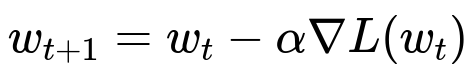
Here, w_{t} represents the parameters at iteration t, alpha is the learning rate, and L(w_{t}) is the loss function evaluated at w_{t}. The gradient term nabla L(w_{t}) in the equation is an approximation of the full gradient if we are doing stochastic gradient descent (often computed on a single or small batch of examples), but the overall principle is the same.
Considering Convex Problems
In a convex scenario, the loss function has the property that any local minimum is also a global minimum. Therefore, if the loss surface is strictly convex, following the gradient should lead to the unique global optimum, assuming the learning rate is chosen carefully and we iterate sufficiently. For strictly convex losses, the gradient direction is theoretically guaranteed to steer us toward that global minimum. However, practical details such as finite step sizes, noisy gradients, and numerical precision can affect the exact path taken. Nonetheless, in the idealized sense, the gradient does indeed consistently guide us toward the global solution.
Considering Non-Convex Problems
When the problem is non-convex, the shape of the loss landscape can be exceedingly complicated, with many local minima, saddle points, and flat regions. The gradient in these domains still directs you in a direction of locally decreasing loss, but it does not guarantee that this direction leads to the global optimum. Instead, it leads to a point where the local slope is minimized. This point may be:
A local minimum, which could be suboptimal.
A saddle point, which in high-dimensional spaces can be common.
A plateau or an area where the gradient becomes small, yet the solution is not truly optimal.
Therefore, in non-convex settings, the gradient does not necessarily carry you to the global optimum; rather, it simply points in a locally descending direction.
Stochastic Nature of SGD
One important aspect of SGD is that it uses noisy gradient estimates. This randomness can sometimes help escape shallow local minima or saddle points by adding a small amount of “noise” to the update direction. Although it does not guarantee reaching the global optimum, it can provide enough stochastic exploration to find a decent local region, often good enough in practice. Still, for highly non-convex tasks, there is no absolute assurance that SGD will consistently converge on the best possible solution.
Summary of Key Insights
The short answer is that the gradient in SGD does not always point to the global optimum in every scenario. In convex optimization problems, the gradient direction guides you closer to the global minimum. In non-convex optimization, the gradient points to a local descent path, but it may not align with the direction of the global optimum. Thus, for non-convex objectives, there is no guarantee that you will land at the global extremum.
How Does the Learning Rate Influence Convergence?
Choosing an appropriate learning rate alpha is crucial. If alpha is excessively large, updates can overshoot minima, causing divergence or oscillations. If alpha is too small, convergence might be extremely slow, or the algorithm might get stuck in suboptimal regions. In convex cases, there are theoretical conditions on alpha that ensure convergence to the global minimum. However, in non-convex settings, you can still get stuck in poor local minima or saddle points regardless of your alpha choice.
Follow-up Questions
In practice, does SGD really find global minima for highly non-convex neural networks?
This question arises because neural networks are famously non-convex. Surprisingly, in many large-scale problems, SGD with proper techniques (initializations, regularizations, batch normalization, learning rate scheduling, and so forth) often finds solutions that generalize well. Research suggests that many modern neural networks have loss landscapes with vast "flat" minima that offer good generalization. Even though these minima are not necessarily the global minima, they can still provide competitive performance in real-world tasks.
How do momentum-based methods affect the direction of the gradient?
Momentum techniques like classical momentum or Adam accumulate moving averages of past gradients. This approach can accelerate convergence in directions where gradients consistently point in a similar direction, and it can help navigate small local minima or saddle points. Nevertheless, momentum-based methods still do not guarantee reaching the global optimum; they can, however, assist in smoothing out noisy updates and may escape certain kinds of bad local minima.
Could second-order methods offer stronger guarantees of finding global minima in non-convex settings?
Second-order approaches such as Newton’s method or quasi-Newton methods examine curvature information to refine the search direction. While second-order techniques can provide faster convergence for convex problems and better local search behaviors in non-convex landscapes, they still do not guarantee global optimality in general non-convex settings. The computational expense of approximating or inverting large Hessian matrices also makes them challenging to apply to modern deep networks.
Do saddle points or plateaus cause more problems than local minima?
In many high-dimensional spaces, saddle points can be more prevalent than local minima. Plateaus (areas where gradients are nearly zero but are not true minima) can also slow progress drastically. When faced with these issues, techniques such as careful initialization, batch normalization, or even adding noise to the gradients (e.g., larger batch size with dropout) can help the optimization process eventually move on to more promising regions.
Overall, the gradient in SGD is an invaluable signal for iterative parameter updates, but it is not a guarantee of reaching a global solution for non-convex tasks. Instead, it is a mechanism for systematic local improvement that, combined with the randomness of sampling mini-batches and other algorithmic design choices, often yields good solutions in practice.
Below are additional follow-up questions
How does the initial parameter setting impact the gradient's ability to lead us to a good solution in non-convex scenarios?
An often-underestimated challenge in non-convex optimization is how you choose your model's initial parameters. If the initial parameters are set near a region of the loss surface with poor local minima or large plateaus, it may be harder to escape or find better basins of attraction. Conversely, starting in a region with more favorable contours can accelerate convergence toward useful minima. For practical deep learning models, techniques like Xavier or Kaiming initialization attempt to balance the scale of inputs and outputs across layers so that gradients neither vanish nor explode. In deeper networks, small differences in initialization can compound over many layers. This is particularly evident in Recurrent Neural Networks or very deep Convolutional Neural Networks, where suboptimal initialization might lead to vanishing or exploding gradients. Additionally, random seeds can cause significantly different paths in the parameter space, especially with stochastic gradient updates. Therefore, multiple random initializations can be used as a hedge against landing in a suboptimal region of the loss landscape.
Does mini-batch size affect our ability to escape local minima, and what are the potential pitfalls when choosing very large or very small batches?
In stochastic gradient descent, the size of the mini-batch can critically shape the learning trajectory. Small batches introduce higher variance in the gradient estimates. That additional noise can act as a natural perturbation, helping the model escape shallow local minima or saddle points. However, a pitfall of using very small batches is that the updates can become highly noisy, potentially causing instability, slower effective convergence, or a need for more careful hyperparameter tuning (like adjusting the learning rate). On the other hand, very large batches produce gradients with lower variance, which can lead to faster per-iteration convergence, but might also get stuck in narrower, sharper minima. Sharp minima often generalize worse than flatter minima, though this tendency can depend on the specific architecture and regularization in use. Another subtle pitfall is that large-batch training typically requires scaling the learning rate, and if not done appropriately, the optimization may fail to converge or might do so very slowly.
How do adaptive learning rate algorithms (e.g., Adam, RMSProp) influence the gradient direction differently compared to vanilla SGD?
Adaptive optimizers such as Adam or RMSProp rescale the learning rate based on historical gradient magnitudes for each parameter. This can help correct for ill-conditioned loss landscapes where some parameters might otherwise receive excessively large or small updates. While this adaptivity can accelerate training and make hyperparameter tuning more forgiving, it also introduces its own pitfalls. For instance, Adam’s faster early progress in non-convex problems can cause it to skate over shallow minima more readily. Moreover, some research suggests that adaptive methods might favor local minima that generalize slightly less effectively compared to those found by vanilla SGD with momentum, though such effects vary widely and are not universal. Another subtlety is that hyperparameter choices in adaptive methods (like the beta parameters in Adam for exponential moving averages) can drastically alter the effective shape of the optimization trajectory, and small changes can have large downstream effects on final performance.
When might gradient-based methods lead to a deceptive sense of convergence in non-convex problems?
A deceptive sense of convergence can arise if the gradient norm becomes small, yet you are actually in a plateau rather than a true local minimum. In high-dimensional spaces, plateaus or saddle plateaus can have very small gradients for large contiguous regions of parameter space, causing many gradient-based algorithms to appear as if they have converged. Moreover, non-stationary data distributions or poor error metrics can mask the reality that improvements are still possible. For instance, you might see minimal improvement in training loss while the validation or test metrics slowly drift. This can happen if your training set is not representative, leading you to “converge” to a local optimum that does not generalize. A thorough approach is to monitor multiple indicators, including training and validation loss curves, gradients, and possibly higher-order metrics or domain-specific performance indicators to detect whether you have reached genuine convergence or just a deceptive plateau.
How can gradient clipping help avoid problematic gradient directions, and what potential issues might it introduce?
Gradient clipping imposes an upper bound on the norm or absolute value of gradients before applying an update. This technique is especially crucial in Recurrent Neural Networks or any architecture susceptible to exploding gradients. By limiting the maximum gradient magnitude, you keep your parameter updates bounded, preventing unstable parameter changes. However, indiscriminate clipping can also mask real differences in gradient magnitude, effectively flattening out the signals you want to use for learning. If clipping is set too aggressively, the model might underfit because it is not adjusting the weights enough in each update step. On the other hand, setting the clipping threshold too high might fail to mitigate exploding gradients. In addition, gradient clipping does not solve the fundamental optimization complexities; it merely addresses the symptom of large updates. Thus, the interplay between the model architecture, learning rate, and clipping threshold must be tuned carefully.
In what ways do data preprocessing and feature scaling influence the reliability of gradients in leading us toward optimal solutions?
Data preprocessing and feature scaling can have a marked effect on the geometry of your loss surface. For instance, if some features have extremely large values and others are very small, the gradient can become ill-conditioned. The optimizer may struggle to navigate directions associated with large-scale features while ignoring or under-updating those associated with small-scale features. Standardizing or normalizing data, or using batch/layer normalization in deep networks, often makes the surface more tractable for gradient-based methods. A potential pitfall, however, is applying overly simplistic preprocessing techniques that might remove valuable structure from the data. Moreover, in real-world scenarios with streaming data, the distribution might shift, invalidating your initial preprocessing assumptions. In that case, the gradient directions you computed can become outdated or misleading, necessitating more dynamic normalization procedures or adaptation strategies.
How does partial or noisy labeling in the dataset affect the gradient direction in SGD, and what are methods to mitigate its impact?
In many real-world cases, labels can be noisy or incomplete. This noise translates into the gradient estimates, possibly pushing updates in directions that are suboptimal or entirely misleading. For example, a consistent fraction of incorrectly labeled data can lead the model to overfit those erroneous labels, making it harder to converge on the correct patterns in the data. Mitigation techniques include:
Label smoothing, which softens hard labels to reduce overconfidence in any single data example.
Robust loss functions that are less sensitive to outliers or label errors.
Active learning approaches that attempt to correct dubious labels.
Semi-supervised or self-supervised methods that exploit large unlabeled datasets to learn representations resilient to label noise.
One subtlety here is that mild label noise sometimes acts like a form of regularization, preventing the model from overfitting completely. However, excessive noise may degrade performance irrecoverably unless suitable countermeasures are in place.
If different local minima yield similar training loss, how do we differentiate which minimum is “best” for real-world performance?
When multiple regions in the parameter space produce nearly the same training loss, the question becomes how they generalize. It is possible that certain minima lead to better performance on unseen data (a phenomenon often referred to as “flat minima” providing better generalization). To differentiate them, one can:
Evaluate on a validation or hold-out test set to see which solution generalizes best.
Inspect the "sharpness" vs. "flatness" of the minima, although this is more of a research-level diagnostic than a day-to-day practice.
Use ensemble methods that combine multiple local minima, thereby averaging their parameters or outputs to potentially achieve improved robustness and performance.
Conduct domain-specific checks (e.g., confusion matrices, F1 scores for classification, or other business metrics) to see if a particular local minimum is superior in the relevant real-world sense.
A pitfall is that focusing solely on training or validation accuracy might obscure other important practical criteria, such as computational cost, interpretability, or fairness metrics.
How do irregular or unbalanced data distributions interact with gradient-based optimization in non-convex models?
When classes or groups in the dataset are highly imbalanced, the gradient may be dominated by the majority class. The model can learn to ignore minority classes or subtle patterns just to minimize overall loss, effectively driving the gradient in a direction that benefits the majority but fails for the minority data. Additionally, real-world data distributions might be long-tailed or subject to concept drift, complicating the assumption that a single global minimum is equally optimal across all classes. Methods to address these pitfalls include:
Oversampling minority classes or undersampling majority classes.
Utilizing weighted loss functions that amplify the importance of underrepresented classes.
Using specialized architectures or multi-task learning setups to balance objectives across subgroups. These interventions help the gradient reflect the broader set of objectives, rather than skewing toward a single global optimum that might be suboptimal for certain classes.