
ML Interview Q Series: In what ways do deep neural networks overcome or alleviate the problems typically referred to as the "curse of dimensionality"?


📚 Browse the full ML Interview series here.
Comprehensive Explanation
Deep neural networks can handle very high-dimensional inputs more effectively than many traditional methods, and they do so by leveraging several core principles: representation learning, hierarchical feature extraction, parameter sharing, and leveraging the manifold hypothesis. Instead of trying to directly learn a function that maps from a high-dimensional input space to an output, deep architectures build increasingly abstract and disentangled representations. By composing layers of parameterized transformations and non-linear activations, they effectively reduce and restructure the input space, mitigating the curse of dimensionality.
One way to see this is through the compositional nature of neural networks. A deep network applies multiple transformations one after another, each layer capturing increasingly higher-level structure. A typical feed-forward network can be summarized by the following composition of functions, where each layer’s function is parameterized by weights and biases and applies a non-linear activation:
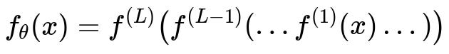
In this expression, x is the input vector, f^{(l)} represents the transformation at layer l, and \theta collectively denotes all learnable parameters across all layers. Each f^{(l)} typically takes the form \sigma(W^(l) * input + b^(l)) in a text-based expression (where W^(l) and b^(l) are layer-specific weight matrices and bias vectors, respectively, and \sigma is a non-linear function such as ReLU or sigmoid). Deep networks effectively learn to re-map the input space into a sequence of feature spaces where each dimension can correspond to a semantically meaningful feature. This layered approach can dramatically reduce the complexity of the problem, thereby helping to combat the curse of dimensionality in practice.
Key Reasons Deep Networks Resist the Curse of Dimensionality
Hierarchical Feature Extraction. Instead of manually engineering features in high-dimensional spaces, deep networks internally learn multi-scale representations that often follow a hierarchy: simple edges or local patches in the early layers, and more complex patterns or objects in deeper layers. By capturing local patterns that repeat across different positions and levels of abstraction, the network can exploit statistical regularities to reduce the effective dimensional complexity.
Parameter Sharing. In convolutional and recurrent architectures, weights are shared across multiple parts of the input. In a convolutional neural network, the same set of filters is applied across different spatial locations, drastically lowering the number of free parameters. This approach means we do not blow up the parameter count solely because of a larger input dimension. For recurrent models, the same transition weights are reused across time steps. Both these strategies help mitigate high-dimensional parameter blow-up.
Manifold Hypothesis. Real-world high-dimensional data (images, speech signals, text) are commonly believed to lie on lower-dimensional manifolds embedded in the high-dimensional input space. Deep networks (especially those with convolutional layers or other structural constraints) can learn mappings that unravel these manifolds, reducing the dimensional complexity that the network must learn to represent. This helps them generalize better even when data is high-dimensional, because the data effectively occupies a smaller volume in that large space.
Effective Function Approximation. Deep networks are universal function approximators when given sufficient capacity and training data. By layering functions, they can approximate a wide variety of high-dimensional functions without requiring an exponential growth in parameters. Their ability to factorize complex functions into simpler, composable building blocks helps them learn efficiently in high dimensions.
Regularization and Generalization Techniques. Methods like batch normalization, dropout, weight decay, or skip connections provide ways to regularize the model, allowing it to learn robustly from high-dimensional data without succumbing to overfitting. This also indirectly helps resist the curse of dimensionality by guiding the network to learn more generalizable and compressed representations of the data.
How the Manifold Assumption Helps
Many data sources—images, text, audio—are not uniformly distributed in their very high-dimensional raw input space. Instead, they lie on much lower-dimensional manifolds. Neural networks with appropriate architectures learn representations aligned with these manifolds. By focusing on relevant directions in the data space (the manifold), the network sidesteps the empty vastness of the entire high-dimensional space, which is the root cause of the curse of dimensionality.
Follow-up Questions
Could you explain how parameter sharing specifically helps reduce the effective dimensionality?
Parameter sharing ensures that not every new part of the input demands its own dedicated set of weights. In convolutional neural networks, for example, the same filters slide over different spatial locations, leading to far fewer parameters than if each location had its own filter set. This means the parameter space (which could be considered part of the "dimensional" burden) grows much more slowly, making the model more efficient and less prone to overfitting. Additionally, it leverages the assumption that features learned at one location could be useful in others, further lowering the difficulty of extracting meaningful representations in high-dimensional inputs.
Is the curse of dimensionality ever still a concern for deep networks?
Yes, it can be. While deep networks handle high-dimensional data better than many traditional approaches, the curse of dimensionality remains relevant when:
Large-Scale Data Is Unavailable. When sufficient training data is not available, even a well-structured neural network might struggle to learn a good representation in very high dimensions.
Uninformative Features. If the data is extremely sparse or does not lie on a lower-dimensional manifold, the network’s advantage is less pronounced. It will require either specific architectural constraints or domain-specific knowledge.
Excessive Capacity. Very large networks with insufficient regularization and data can still overfit to high-dimensional inputs, showing that the curse of dimensionality can strike if not carefully managed.
How do we know the manifold assumption holds?
In many real-world tasks (images, speech, language), empirical evidence shows that data samples are concentrated in regions that have significantly fewer degrees of freedom than the raw dimension suggests. Techniques like dimensionality reduction (PCA, t-SNE, autoencoders) show that low-dimensional embeddings often capture most of the variation. However, it is typically an empirical observation rather than a guaranteed law. That said, neural networks—especially convolution-based architectures—tend to do well precisely because they exploit such assumptions, and hence, it works well in practice for large classes of problems.
Does having deeper networks always mean we avoid the curse of dimensionality better?
Deeper is not always strictly better, because other factors (data quantity, model regularization, optimization stability) play major roles. Depth can help represent functions more compactly by factoring them into a sequence of simpler transformations. However, increasing depth blindly without enough data or proper hyperparameter tuning can lead to vanishing gradients, overfitting, or training instability. In well-designed networks, deeper architectures tend to be more expressive and are often more sample-efficient, but it is not a panacea if other design considerations and data requirements are not met.
Could shallow networks require exponentially more parameters to match deep networks?
Yes. Theoretical results suggest that certain classes of functions that are representable in a compact form by a deep network might require exponentially more neurons or parameters in a shallow network. This exponential blow-up ties into the curse of dimensionality. By employing depth, we factorize the function into a hierarchy, allowing the network to share and reuse intermediate representations. This factorization is key in reducing the parameter count needed to represent complex high-dimensional functions, thus mitigating the curse of dimensionality.
Can transfer learning also help handle high-dimensional data?
Absolutely. Transfer learning leverages knowledge learned from a large source dataset and applies it to a new task, often in the same or similar input space. This approach effectively gives the model a head start, where it does not have to learn all features from scratch in the new high-dimensional domain. Because many features from the source task transfer well to the target domain, the model needs less data for the new task, thus easing the difficulties associated with high dimensionality and data sparsity.
Is there a limit to how large the network can be before the dimensionality becomes an issue again?
If we keep increasing the number of parameters without corresponding increases in data and appropriate regularization, the model may eventually overfit, or training could become infeasible. There is also a practical limit in terms of computational resources and memory. In reality, engineers balance these concerns with architectural design choices—like skip connections, batch normalization, or specialized layers (e.g., attention mechanisms in transformers)—to allow very large networks to train effectively. But in principle, if the network vastly outscales the dimensional manifold of the data, generalization may suffer unless massive data or specialized techniques are used.
Could regularization be viewed as a way to fight the curse of dimensionality?
Yes. Regularization injects constraints or priors that shape how the model explores the parameter space. Methods like dropout, L2 weight decay, or early stopping effectively reduce how freely the network can learn arbitrary high-dimensional mappings, nudging the learned function to be smoother or sparser. This helps the model concentrate on more meaningful and generalizable patterns, thereby reducing issues that arise when trying to learn from extremely high-dimensional data with limited samples.
These strategies, combined with carefully designed architectures, are the critical ways that deep neural networks mitigate the curse of dimensionality and successfully handle extremely large input spaces.
Below are additional follow-up questions
When might a simpler model still outperform a deep neural network in very high-dimensional settings?
Even though deep neural networks can handle high-dimensional data effectively in many scenarios, there are cases where a simpler model might still be preferable. One key factor is the size and nature of the available dataset. If the dataset is too small, deep neural networks can overfit quickly in high dimensions unless there is a very strong regularization regime and well-tuned hyperparameters. Simpler models like linear or tree-based methods might have fewer parameters and thus a smaller variance in their estimations, potentially leading to better performance. Another situation arises if the underlying data distribution is fairly linear or does not require the representational capacity of deep architectures. In such cases, a well-regularized simpler method can often converge faster and generalize adequately without the added complexity.
Pitfalls include failing to realize that some domains do not benefit from hierarchical feature representations. If the data does not exhibit structured patterns (e.g., repeated local features or hierarchical compositionality), the advantages offered by deep networks—like parameter sharing and building progressively abstract representations—may not materialize. It is also possible that the engineering overhead and tuning complexity for a deep network exceed the gains in accuracy, making simpler approaches more practical.
How do interpretability and explainability factor into handling high-dimensional data?
While deep networks may help mitigate the curse of dimensionality, the internal learned representations can be challenging to interpret. In very high-dimensional spaces, the network’s layers extract features that may not have direct human interpretations. This creates a tension: on one hand, deep models can provide state-of-the-art performance by capturing complex relationships; on the other hand, the transformations they learn can obscure exactly how specific features or sub-dimensions affect predictions.
In real-world applications, especially in regulated industries (like healthcare or finance), the ability to explain predictions can be critical. In high-dimensional domains, these demands become more challenging, leading practitioners to adopt techniques such as layer-wise relevance propagation, Shapley values, or attention-based introspection. These methods help reveal which input dimensions or learned features drive the model’s outputs. A pitfall arises when interpretability is mandated but not accounted for during model design: building a very deep or complex architecture without regard to how it might later be interpreted can cause friction or require extensive post-hoc analysis that may be inconclusive.
How do autoencoders help reduce dimensionality and combat the curse of dimensionality?
Autoencoders learn a compressed representation by forcing the input data through a bottleneck layer with fewer neurons than the original input dimension. In doing so, the network extracts essential features that reconstruct the data as accurately as possible. By capturing the most salient factors of variation in the data, the autoencoder effectively focuses on a lower-dimensional manifold where the relevant structure lives. This is particularly useful for visualization, noise reduction, or as a pretraining step in various tasks.
However, there are pitfalls. If the autoencoder’s capacity is too large and it is insufficiently regularized, it may simply memorize or copy the input, failing to learn a truly compressed representation. Another common issue is that the learned latent dimension might not align with a meaningful subspace for downstream tasks if the reconstruction loss does not incentivize the right form of structure. A variant like the Variational Autoencoder (VAE) constrains the latent space further to be a continuous, well-defined manifold, helping maintain a more robust representation in high-dimensional spaces.
Can data augmentation techniques alleviate the curse of dimensionality, and under what circumstances might they fail?
Data augmentation artificially increases the diversity and volume of training samples by applying transformations (e.g., rotations, flips, color jitter) that do not change the semantic meaning of the data. When handling high-dimensional inputs like images, these augmentations can be crucial in helping deep networks generalize. They effectively increase the coverage of the input space without requiring entirely new real data.
However, these methods can fail or even be detrimental if the chosen transformations are not valid for the specific problem or domain. For instance, rotating an image of text or flipping a medical scan might distort the underlying content in ways that mislead the model. Additionally, in extremely high-dimensional domains where meaningful transformations are hard to define (e.g., arbitrary sensor readings, genetic data), naive augmentation strategies may not help capture the real-world variability. In such cases, blindly applying augmentation can degrade performance if it introduces artifacts or unrealistic samples.
Do specialized architectures, such as Graph Neural Networks (GNNs), mitigate the curse of dimensionality in certain data types?
Yes, GNNs can be particularly effective when the data has an inherent graph structure. Traditional approaches to high-dimensional graph data might attempt to flatten adjacency matrices or node features, leading to huge input vectors and sparse signals. GNNs share parameters across nodes, learn localized aggregation rules (e.g., message passing), and can generalize well, especially on graph-structured data from domains like social networks, molecular graphs, or recommendation systems.
A potential pitfall is when the graph structure itself is not well-defined or is too noisy. If there is no meaningful way to express local connectivity, then a GNN’s advantage (the ability to propagate messages through node connections) may be irrelevant or could even introduce confusion in the representations. Furthermore, if the graph is extremely large or dynamic (e.g., nodes and edges constantly changing), computational scalability and memory usage may become significant challenges, requiring distributed training or approximate inference methods.
How do high-dimensional optimization challenges, such as local minima or saddle points, factor into deep network training?
In high-dimensional parameter spaces, local minima are often less of an issue than saddle points or plateaus, where gradients are very small along certain dimensions and the training gets “stuck” temporarily. Deep networks are typically resilient to poor local minima because of overparameterization—many different parameter configurations can yield similarly low training loss. However, navigating saddle points can slow down training and cause unpredictability in convergence.
One subtle point is that overparameterized networks with huge dimensional parameter spaces can exhibit favorable geometry, making true local minima less common. Yet, poor initialization or improperly tuned learning rates can exacerbate the negative effects of saddle points, causing training to plateau. Methods like learning rate schedules, adaptive optimizers (Adam, RMSProp), or advanced second-order methods can help. Another pitfall is that some complex architectures, if not carefully designed, may create optimization landscapes rife with saddle regions—particularly if there are recurrent or cyclical dependencies in the computation graph.
What about generative models that attempt to capture the full data distribution in high-dimensional spaces?
Generative models like Generative Adversarial Networks (GANs), Variational Autoencoders (VAEs), or diffusion models all aim to represent the probability distribution of high-dimensional data. They mitigate the curse of dimensionality by learning a compressed latent space from which samples can be drawn. In practice, these models assume the data is concentrated on lower-dimensional manifolds, enabling them to learn complex distributions without enumerating the entire huge input space.
Pitfalls include mode collapse in GANs, where the generator fails to capture the diversity of the data distribution. VAEs may produce blurry samples if the model’s capacity or loss function is not well-tuned. Diffusion models require careful balancing of the forward and reverse processes. In high-dimensional domains, these challenges can be exacerbated if the model is not sufficiently regularized or if there is not enough data to cover the manifold comprehensively. The training process can also become computationally expensive, requiring large-scale hardware and careful hyperparameter tuning to ensure stable and meaningful convergences.