
ML Interview Q Series: In which ways can Genetic Algorithms be used to refine a Deep Learning classifier’s architecture?


📚 Browse the full ML Interview series here.
Comprehensive Explanation
Genetic Algorithms are population-based search and optimization methods inspired by natural evolution. Each potential solution to the architecture and hyperparameters of a Deep Learning model can be treated as an individual in a population (often called a chromosome). Over several iterations (generations), these individuals compete based on their performance, and the top performers produce offspring for subsequent generations.
Genetic Algorithms begin by encoding the neural network’s architecture and hyperparameters (such as number of layers, number of neurons in each layer, activation functions, or learning rates) into a representation suitable for genetic operations. This could be a list or vector in which each entry corresponds to a choice (for example, how many filters in a convolutional layer, or which activation function to use). Once the population of candidate solutions is initialized randomly, we measure performance on a given dataset. The key is to choose a meaningful fitness function that accurately assesses the classifier’s performance.
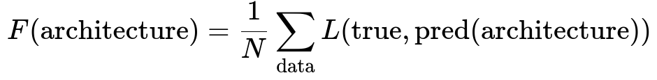
Where F(architecture) is the fitness of a particular network design, N is the total number of data samples, and L(true, pred(architecture)) is a loss evaluation of the network with the given architecture on a sample. The lower the loss, the higher the fitness. Here we usually transform the loss into a score or some performance measure such as accuracy or F1 score for direct maximization.
In practice, Genetic Algorithms involve four main operations:
Selection: Pick highly fit architectures based on their performance. Crossover: Combine parts of two selected architectures to form offspring. Mutation: Randomly modify parts of the offspring (e.g., swap neurons in a layer or alter the number of filters). Replacement: Insert the newly created offspring into the population, often replacing less fit individuals.
By iterating these steps for multiple generations, the population converges (or partially converges) toward architectures that yield better and better results. This approach can uncover non-intuitive configurations that manual tuning or grid search methods might miss.
Practical Implementation
One must decide on how to represent the architecture. For example, we might encode a convolutional neural network as a sequence describing the number of convolutional layers, filter sizes, strides, activation functions, fully connected layers, and so on. Each encoded architecture is trained for a specific number of epochs (often fewer epochs are used in early generations to save time) and is then evaluated on a validation set to obtain its fitness value.
Another critical element is controlling mutation rates, selection pressure, and population sizes to balance exploration and exploitation. If the mutation rate is too high, we might lose promising architectures; if it is too low, the search might get stuck prematurely.
Example Python Code
Below is a simple conceptual code example of how one might structure a Genetic Algorithm for a neural architecture search using Python-like pseudocode. This example shows the high-level flow rather than a fully optimized production pipeline.
import random
import numpy as np

# Assume we have a function that can build, train, and evaluate a model
# given an architecture representation, returning a fitness score

def evaluate_architecture(architecture):
    # Build the model (e.g., PyTorch or TensorFlow)
    # Train the model for a small number of epochs
    # Return a validation performance metric as fitness
    return fitness_score

def crossover(parent1, parent2):
    # Example single-point crossover
    crossover_point = random.randint(1, len(parent1) - 1)
    child1 = parent1[:crossover_point] + parent2[crossover_point:]
    child2 = parent2[:crossover_point] + parent1[crossover_point:]
    return child1, child2

def mutate(architecture, mutation_rate=0.1):
    # Randomly change some parts of the architecture
    new_arch = []
    for gene in architecture:
        if random.random() < mutation_rate:
            # Apply some random change to the gene
            mutated_gene = some_mutation_function(gene)
            new_arch.append(mutated_gene)
        else:
            new_arch.append(gene)
    return new_arch

def genetic_search(pop_size=20, generations=10):
    # Initialize random population
    population = [random_architecture() for _ in range(pop_size)]

    for gen in range(generations):
        # Evaluate fitness
        fitness_values = [evaluate_architecture(arch) for arch in population]

        # Sort population by fitness (descending if higher is better)
        population = [arch for _, arch in sorted(zip(fitness_values, population), reverse=True)]

        next_generation = []

        # Always keep some of the best
        elite_size = pop_size // 5
        next_generation.extend(population[:elite_size])

        # Generate offspring
        while len(next_generation) < pop_size:
            parent1, parent2 = random.choices(population[:10], k=2)
            child1, child2 = crossover(parent1, parent2)
            child1 = mutate(child1)
            child2 = mutate(child2)
            next_generation.append(child1)
            if len(next_generation) < pop_size:
                next_generation.append(child2)

        population = next_generation

    # Return the best individual
    best_arch = population[0]
    return best_arch

best_architecture = genetic_search()
print("Best architecture found:", best_architecture)
Potential Pitfalls
One common challenge is the computational cost. Training deep neural networks repeatedly can be expensive, so often strategies such as early stopping, partial training (training for fewer epochs), or smaller proxy tasks are used to reduce evaluation time.
Overfitting to the validation set is another concern, especially if the dataset is small or if the search runs for many generations. Keeping a separate test set untouched during the search is a wise strategy.
Poor encoding strategies can lead to large parts of the search space becoming inaccessible or to a representation that is too constrained. Designing a flexible representation is crucial to explore the space properly while maintaining constraints that prevent infeasible or incompatible architectures.
Follow-Up Questions
How do we ensure diverse architectures are explored rather than converging too quickly?
Maintaining diversity in the population is essential. One approach is to use mechanisms like tournament selection or rank-based selection instead of purely picking top performers, thereby allowing less fit but different architectures to continue. Adjusting crossover and mutation rates also helps. If all promising individuals share too many traits, injecting random mutations or using diversity-preserving schemes (like crowding or niching) can avoid premature convergence.
What is a suitable strategy to reduce the computational overhead during the search?
It is useful to train models for fewer epochs when evaluating fitness in early generations, since poorly performing architectures can be discarded without exhaustive training. Another approach is to use smaller versions of the dataset or approximate accuracy measures that correlate well with the final metrics. Once the population narrows to a smaller set of high-potential architectures, one can perform more thorough training.
How does this approach compare to other Neural Architecture Search methods?
Genetic Algorithms can be more interpretable and easier to integrate with custom constraints. However, they might be slower than gradient-based search techniques such as Differentiable Architecture Search (DARTS) or reinforcement learning approaches for neural architecture search. Still, GAs have the advantage of exploring a broader range of structural variations, especially if the representation is designed to allow free-form changes, and they do not require differentiability of the search space.
What are some best practices for encoding the neural architecture in a Genetic Algorithm?
Encodings should be designed to be compact enough to be mutated and recombined but flexible enough to represent different choices in layer type, size, and hyperparameters. One common approach is to have each gene represent a layer or block, where the block specification includes layer depth, filter dimensions, or activation type. Another strategy is to encode a directed acyclic graph representation, which is more flexible but requires careful design of crossover and mutation operations to ensure valid architectures.
When do we decide to stop the Genetic Algorithm?
Common stopping criteria include a fixed number of generations or a threshold on fitness improvement. If the top performing architectures do not improve beyond a certain margin for multiple generations, this might indicate convergence. However, it is often beneficial to keep a separate “patience” parameter so that we do not halt prematurely; if improvement is stagnant for too long, it may be time to stop and finalize the best discovered architecture.
Below are additional follow-up questions
How can we handle massive search spaces when designing Genetic Algorithms for Deep Learning architectures?
Genetic Algorithms inherently explore vast search landscapes because every possible combination of layers, activation types, and hyperparameters can be considered part of the search space. When dealing with large-scale architectures, the risk is that the population-based approach might become too computationally expensive. This happens because each individual (architecture) must be trained to evaluate its fitness, and as the space of candidates grows, so do the training requirements.
One practical approach is to apply staged or hierarchical searches:
• Staged Search: Begin with smaller models or fewer hyperparameters, and once a promising subset of the search space is identified, expand the search to more complex architectures. • Surrogate Models: Use a cheaper approximation of the fitness function. This might involve building a smaller network that is faster to train and acts as a proxy for the larger, final model. • Early Stopping and Partial Training: Rather than fully training each candidate, train every model for a limited number of epochs or until early stopping criteria is met. Discard architectures that do not exhibit promising early trends.
A subtle pitfall arises if the surrogate or partial training strongly deviates from final performance. For instance, certain architectures might take longer to reach their full potential. As such, one must be cautious: partial training can bias against architectures that have slower learning curves but eventually surpass others in the long run.
What if we want to incorporate domain-specific constraints or prior knowledge into the Genetic Algorithm?
In many real-world scenarios—especially in areas like medical imaging or autonomous driving—there can be constraints on the model size or real-time inference requirements. Genetic Algorithms can incorporate these constraints directly into the encoding or the fitness function.
• Constraint in Encoding: If a problem demands the network to fit into a specific computational budget (e.g., less than 10 million parameters), the encoding can disallow any layer combination that exceeds this limit. Similarly, if certain layers are known to be beneficial for a domain (for instance, residual blocks in computer vision tasks), the encoding can prioritize or always include these components. • Modified Fitness Function: In addition to accuracy, incorporate a penalty term for larger models, or a term that rewards faster inference time. This transforms the problem into a multi-objective optimization, where the algorithm searches for solutions that balance performance, parameter count, and latency.
The main subtlety here is finding the right balance in multi-objective settings. Overly strict penalties might discourage exploration of high-performing but larger models. Conversely, lenient penalties could lead to massive networks that might not be feasible in production.
How do we manage randomness in Genetic Algorithms to ensure reproducibility of results?
Genetic Algorithms rely on random initialization, selection, crossover points, and mutation events. This can introduce variability in the discovered architecture. While in research settings we often set fixed random seeds to reproduce experiments, in a real-world scenario (especially in distributed or parallel settings) some degree of nondeterminism is inevitable.
• Fixed Random Seeds: In single-threaded environments, you can often fix the seed to get identical runs. • Tracking Lineage: Logging every individual architecture and the random choices that led to its creation is critical. This helps trace back exactly how a model was formed. • Statistical Validation: Run multiple Genetic Algorithm trials, each with different seeds, and observe the variance in final results. If the variance is large, it might mean the population size or number of generations is insufficient, or the search space is excessively large.
A hidden risk is that reproducibility might degrade as soon as you move to multi-threaded or GPU-based training, because parallel floating-point operations might vary slightly. While such minor numeric differences might not matter for large-scale exploration, you should still be aware that perfect bitwise reproducibility is challenging in distributed frameworks.
How do we effectively parallelize or distribute the workload of Genetic Algorithms for large-scale neural architecture search?
Each individual in a Genetic Algorithm population needs to be evaluated independently to measure its fitness. This naturally lends itself to parallel or distributed computing. However, coordinating a distributed search can be intricate:
• Parallel Fitness Evaluation: Assign each candidate architecture to a different GPU or compute node for training. This can drastically shorten the evaluation time per generation. • Synchronized Generations: After all individuals in a generation are evaluated, the results must be aggregated to perform selection, crossover, and mutation. This requires a master node or an orchestration process. • Asynchronous Methods: Another strategy is to allow individuals to enter the population asynchronously, meaning as soon as one candidate is evaluated, it can be selected for crossover without waiting for the entire generation. This keeps the compute resources continuously busy but complicates the notion of a “generation.”
An edge case is if training times differ significantly among architectures—for instance, some have more layers or complex blocks. Then certain GPUs might finish tasks faster, while others take much longer, leading to resource underutilization. Balancing workloads or setting a maximum training epoch can help mitigate these bottlenecks.
How can Genetic Algorithms be adapted if the data distribution changes over time (non-stationary environments)?
In non-stationary environments, data patterns can shift—common in applications like streaming data or evolving user behavior. Traditional Genetic Algorithms assume the fitness function remains consistent, but in dynamic contexts, the same architecture may no longer perform well as data changes:
• Online Evaluation: Continually update the fitness of an architecture as new data arrives. This means re-training or at least fine-tuning the model regularly on the latest data. • Windowed Fitness: Define a window of recent data to evaluate performance, so older data does not bias the fitness measure. • Continuous Evolution: Rather than performing a fixed number of generations, the algorithm can perpetually run, removing poorly performing architectures and introducing new ones as the data distribution shifts.
A tricky pitfall here is model “forgetting.” As new data arrives, older knowledge might be lost if the model is not carefully updated. This can lead to oscillations in fitness scores, where the system continually readapts to new data but forgets older patterns that occasionally reappear.
How would we address multi-objective optimization (e.g., classification accuracy vs. interpretability or accuracy vs. memory usage)?
In many real-world scenarios, it is insufficient to optimize only for accuracy or loss. Memory constraints, inference latency, interpretability, or energy consumption can be critical design factors:
• Pareto Front: Instead of a single fitness measure, we maintain a set of solutions along a Pareto front, where each solution is considered optimal if no other solution is strictly better in all objectives. • Weighted Sum Approach: Combine multiple objectives into one scalar measure by applying weights, for instance: fitness = accuracy_score - alpha*(memory_usage). This is simpler but depends heavily on the choice of alpha. • Domination-Based Selection: During selection, architectures that dominate others in all objectives are preferred.
One hidden complexity is that interpretability measures or memory consumption may be non-trivial to compute. For example, interpretability might involve metrics like the number of layers or a specialized measure of explainability. Designing these extra metrics requires domain knowledge, and blindly applying them can yield suboptimal or misleading results.
How do we ensure that learned architectures generalize well instead of overfitting to a particular data split?
Since Genetic Algorithms heavily exploit the fitness metric, overfitting to the validation set can occur if the same partition is used repeatedly. Over many generations, the algorithm might discover architectures that exploit nuances of the validation data without truly improving generalization.
• Multiple Validation Splits: Alternate among multiple validation subsets in different generations, or use cross-validation. • Add Random Noise to Training: Introduce stochastic data augmentations or randomizations so that each architecture experiences slightly different data distributions. • Hold-out Test Set: Reserve a completely separate test set that is never used during the evolution. Assess final candidate architectures only once to estimate true generalization.
A subtle point is that if the validation set is changed too frequently or is too random, the fitness estimates might become noisy, causing the Genetic Algorithm to wander or fail to converge. Balancing stable yet diverse validation methods is key.
In practice, how can we determine a proper population size for the Genetic Algorithm?
Choosing a population size is often a trade-off between exploration and computational resources:
• Larger Populations: Provide greater diversity but are more computationally expensive because each generation requires training more models. • Smaller Populations: Train fewer models each generation, which can speed up each iteration but may lead to premature convergence and lower coverage of the search space.
One strategy is to dynamically adjust the population size based on convergence signals. If improvement stalls, you might increase mutation rates or add new random individuals to reintroduce diversity.
The primary pitfall is that a population that is too small might collapse to a few suboptimal architectures, while an overly large population might be infeasible to evaluate given time or hardware constraints. Monitoring the variance in fitness across individuals helps gauge whether the population remains sufficiently diverse.
How might a Genetic Algorithm solution be combined with a fine-tuning or local search step to further improve results?
After finding a strong candidate with the Genetic Algorithm, local search or gradient-based fine-tuning can refine hyperparameters or architectural details. For instance, if the Genetic Algorithm decides on the number of layers and type of activation functions, one could run a short Bayesian optimization on learning rate or batch size around that architecture to eke out further gains.
However, it is worth noting that local search might lead to solutions that only marginally improve performance, especially if the search space is rugged or the Genetic Algorithm already found a near-optimal configuration. Also, local search methods might overfit to a particular local minimum that is not representative of better designs in adjacent areas of the architecture space.
What metrics or indicators would you track to diagnose issues during evolution?
Population Diversity: If all individuals become too similar too quickly (e.g., standard deviation of gene values across the population is near zero), you risk premature convergence.
Fitness Improvement Rate: Track how quickly the best, average, and worst fitness values improve each generation. If they stagnate, it might be time to increase mutation or reevaluate the search space.
Computational Cost: Monitor training time per individual. If some architectures are too large or complex to train in a reasonable timeframe, you may need to constrain the architecture encoding or adopt partial training strategies.
Generalization Gap: Keep an eye on the difference between training and validation performance. A widening gap indicates potential overfitting.
A subtlety here is that moderate, steady improvements might still yield a breakthrough after several generations, whereas a rapid early improvement might plateau if the search space is not well understood. Balancing short-term performance jumps with long-term exploration is key.