
ML Interview Q Series: Inferring Ball Composition with Conditional Probability After Observing a Draw.
Browse all the Probability Interview Questions here.
Question: Somebody puts eight balls into a bowl. The balls have been colored independently of each other, each one red or white with probability 1/2. This occurs unseen to you. Then you see two additional red balls being added to the bowl. Next, five balls are drawn at random and revealed to be all white. What is the probability that the remaining five balls in the bowl are all red?
Short Compact solution
Define event A as: “Before the two red balls were added, there were exactly 5 white balls and 3 red balls in the bowl.” Define event B as: “When 5 balls are drawn from the now 10-ball bowl, all 5 are white.”
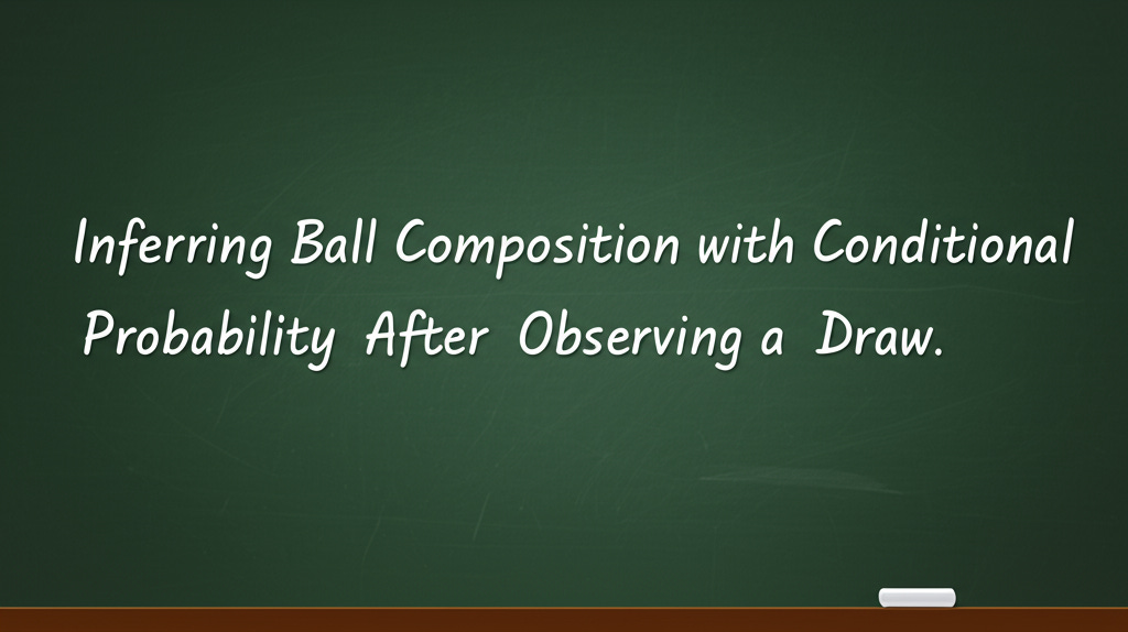
We use conditional probability to find P(A given B). The numerator is the joint probability that there were originally 5 white and 3 red (each ball was red or white independently with probability 1/2) and that all 5 drawn are white after the two extra red balls have been added. The denominator is the total probability that all 5 drawn are white for any possible composition of the original 8 balls. It works out to:
Evaluating the sum in the denominator and simplifying yields the result 1/8.
Comprehensive Explanation
The problem statement can be interpreted as follows:
There are initially 8 balls in a bowl. Each ball is red or white with probability 1/2, independently of the others.
Then 2 red balls are added to the bowl, bringing the total number of balls in the bowl to 10.
Next, 5 balls are drawn from these 10. All 5 drawn are observed to be white.
We want the probability that the remaining 5 balls left in the bowl are all red.
Setting up the events
Let A be the event that among the original 8 balls, there were exactly 5 whites and 3 reds. After adding 2 red balls, the composition would then be 5 white + 5 red = 10 total.
Let B be the event that the 5 drawn balls (from the 10) are all white.
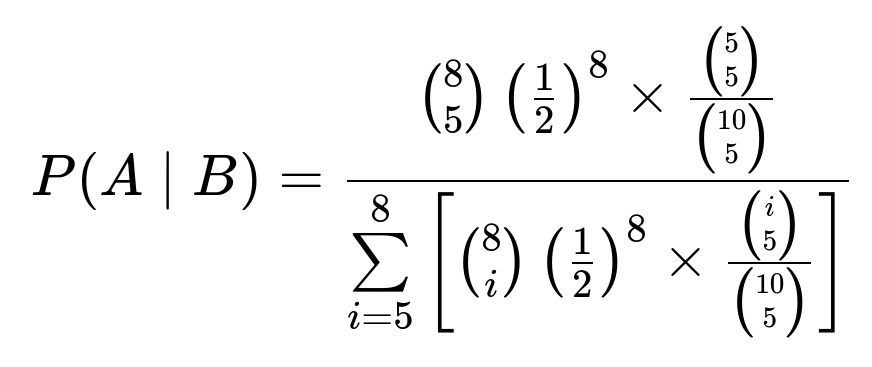
We are looking for P(A given B), which by definition of conditional probability is:
Computing P(A ∩ B)
The probability that exactly 5 of the original 8 balls were white and 3 were red is (8 choose 5) (1/2)^8 because each of the 8 balls is independently red or white with probability 1/2.
Given that scenario (5 white + 3 red originally), we add 2 red balls, so the total becomes 5 white + 5 red = 10.
The probability of drawing 5 white out of those 10 when we pick 5 balls is (5 choose 5) / (10 choose 5), since there are 5 white balls in the bowl and we want all 5 chosen to be white, out of all possible ways of choosing 5 from 10.
Putting this together:
P(A ∩ B) = [ (8 choose 5) (1/2)^8 ] × [ (5 choose 5) / (10 choose 5) ].
Computing P(B)
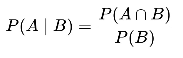
P(B) is the probability that we draw 5 white balls, regardless of how many white and red were in the original 8. We need to consider all possible ways i red balls could appear in the original 8, for i = 0, 1, 2, …, 8. Since we only get 5 whites in the draw if at least 5 of the total 10 balls are white, the relevant i values range from i = 0 (which means 8 white, 0 red) up to i = 8 (which means 0 white, 8 red). However, note that for the event B to occur (5 white are drawn), we must have at least 5 white balls in the final bowl. That means among the original 8, we must have i≥3 red, or equivalently at most 5 white. A simpler approach is to explicitly sum from i = 5 to 8 the relevant probabilities, because i represents the count of white balls (or, equivalently, 8 – i is red). Often one carefully enumerates all compositions that allow at least 5 white in the final mix of 10. The compact formula is:
where i is the number of white balls in the original 8.
The final ratio P(A|B)
Dividing P(A ∩ B) by P(B) (and simplifying the expressions) leads to 1/8. Thus, given that we observed 5 white balls in the draw, the probability that the remaining 5 balls in the bowl are red is 1/8.
Intuitive reason
This result might seem surprisingly small, but remember that there are many ways to have ended up drawing 5 white balls from the mixture. If the original 8 contained more than 5 white balls, that also would make it more likely to see an all-white draw. We specifically need the case of exactly 5 white among the original 8, which is only one part of that entire probability space.
What if you want to verify via simulation?
Here is a brief Python snippet that empirically estimates the probability:
import random

def simulate(num_trials=10_000_00):
    count_event = 0
    for _ in range(num_trials):
        # Step 1: Generate 8 balls (each red=0 or white=1 with p=0.5)
        original = [random.choice([0,1]) for _ in range(8)]
        # Step 2: Add 2 red balls (red=0)
        bowl = original + [0, 0]

        # Step 3: Randomly choose 5
        drawn = random.sample(bowl, 5)

        # Step 4: Check if all drawn are white
        if all(ball == 1 for ball in drawn):
            # Step 5: Check if the 5 remaining in the bowl are all red
            remaining = [ball for ball in bowl if ball not in drawn or drawn.remove(ball)]
            if all(ball == 0 for ball in remaining):
                count_event += 1
    # Probability = P(A ∩ B) / P(B)
    # But we only simulate B's condition, so we need the fraction
    # of times among all B occurrences that A also occurs.

    # The fraction is count_event / total_occurrences_of_B
    # We can do it in a two-pass approach or store partial counts:

    # Let's do a simpler approach: for big simulation, do it in two passes:
    return count_event

def simulate_probability(num_trials=10_000_000):
    b_occurrences = 0
    ab_occurrences = 0
    for _ in range(num_trials):
        original = [random.choice([0,1]) for _ in range(8)]
        bowl = original + [0, 0]
        drawn = random.sample(bowl, 5)
        if all(ball == 1 for ball in drawn):
            b_occurrences += 1
            remaining = [ball for ball in bowl if ball not in drawn or drawn.remove(ball)]
            if all(ball == 0 for ball in remaining):
                ab_occurrences += 1
    # Among the trials in which B occurs, the fraction that also satisfies A is:
    return ab_occurrences / b_occurrences if b_occurrences else 0

prob_est = simulate_probability()
print(prob_est)
For large num_trials, the result will approximate 0.125, which is 1/8.
What if the probability of red or white was not 1/2?
If red or white had different probabilities, say p for red and 1 – p for white, you would adjust the combinatorial factors to reflect that the probability of having i white among the original 8 is (8 choose i) * (1 – p)^i * p^(8 – i). The added 2 red balls remain the same. You would then compute the likelihood of drawing 5 whites conditional on that composition, and sum over i≥5. The methodology remains identical; only the prior distribution on the count of white vs. red in the original 8 changes.
How does conditional probability relate to typical machine learning applications?
In many machine learning tasks, especially Bayesian approaches, you update your belief about the parameters (like the composition of a dataset) after seeing some evidence (like the drawn balls being white). Observing evidence that certain outcomes happen influences your estimate of unknown parameters. This question is a straightforward application of conditional probability: prior belief about the composition, then an update based on the observed data (all white draws).
How could this extend to larger samples?
If you had more balls and more draws, you could use exactly the same framework, but the combinatorial expressions would grow larger. In practice, you might rely on computational methods or approximations (e.g., Bayesian simulation) to handle large numbers of balls or complex distributions.
Are there alternative ways to approach this problem?
An alternative perspective might use Bayes’ Theorem explicitly to compute posterior probabilities for the composition of the 8 original balls, given the observed draw. This is effectively what we did; we just labeled it with conditional probability notation. Another route could involve direct enumeration or simulation as illustrated with the Python code. However, the result would be the same: 1/8.
Below are additional follow-up questions
What if we change the number of balls drawn to a value other than 5? How would this impact the probability calculation?
In the original scenario, 5 balls are drawn and all are white. If instead some other number k of balls are drawn and observed to be white, the approach stays the same but the binomial coefficients and summations in the conditional probability formula change accordingly. Specifically:
We would let A be the event that the original 8 balls have the composition necessary to yield the scenario of interest (e.g., exactly 5 white, 3 red if we still want the remainder to be a certain color combination).
We would let B be the event that
kdrawn balls are all white, for instance.Then we compute P(A|B) = P(A ∩ B) / P(B) by summing over all possible ways the original 8 balls might be distributed in terms of red/white.
A potential pitfall: As k approaches the total number of balls in the bowl, the chance of seeing “all white” is impacted more dramatically by compositions that have many white balls. This means small differences in composition assumptions can drastically change P(B). In extreme cases (like drawing all but one ball), the probabilities can become trivial (i.e., if you draw 9 out of 10 balls, seeing them all white severely restricts how many red could have been in the original set).
An edge case: If k is larger than the number of white balls in the entire bowl, then event B cannot occur at all (probability 0). Also, if k=0 (no balls drawn), event B is vacuously satisfied but provides no information to update our belief about the bowl.
How would the probability be affected if the observer had partial information about the draw (e.g., only the count of white balls among the drawn sample, not each individual ball)?
In many real situations, you might only get aggregated information such as “4 out of the 5 drawn balls were white,” without seeing exactly which ones. If you only have partial information, the analysis is similar but you adjust the likelihood of that aggregated outcome. Instead of requiring that all 5 are white, you would compute the probability of exactly 4 white and 1 red (or whatever the partial info is). Then apply Bayesian updates the same way:
Compute P(B) under partial information by summing the probabilities of any composition of the original 8 that can yield the observed “4 white out of 5.”
Compute P(A ∩ B) for the composition of interest A, intersected with that partial observation B.
Take the ratio.
A key subtlety is that aggregated data sometimes loses information about exactly which positions in the sample were white or red. This can make certain compositional inferences less precise, but the fundamental conditional probability approach remains the same.
Pitfall: If the partial information is ambiguous (for instance, you might not even know the exact number of white vs. red, just a range), you need to sum or integrate over all consistent outcomes. Omitting possible consistent outcomes leads to incorrect posteriors.
What if there is a chance that the coloring of the original 8 balls is not truly independent or not a strict 50–50 probability for red vs. white?
In more realistic settings, the 8 original balls might have correlated colors or a different marginal probability for red vs. white. For instance, maybe there is a 60% chance of any ball being red and 40% chance of being white, or some correlation such that typically more reds come together. You would then change the prior distribution P(A) accordingly:
If the red/white probability is p for each ball (and still independent), you would replace (1/2)^8 with p^(number_of_red) (1 – p)^(number_of_white).
If the draws are correlated, you need a joint distribution for the number of red vs. white in the 8 balls.
Pitfall: If you mistakenly assume independence and 50–50 coloring when the real distribution differs, you will get an incorrect posterior probability. In real-world scenarios, correlation (e.g., if balls came from the same batch or if color depends on some external factor) can significantly alter the final probabilities.
Edge case: Perfect correlation could mean either all 8 original balls share the same color or some known ratio. Then the prior probability for each composition might be zero except for specific distributions, radically changing the summation in P(B).
How would the answer differ if the 2 added balls were not guaranteed to be red?
Suppose that instead of “2 red balls were added,” we only know that “2 additional balls are added, each of which is red with probability p and white with probability 1 – p.” Then, we have a more complex problem. The final bowl would contain an uncertain composition from both the original 8 (randomly colored) and the 2 new uncertain balls. The steps become:
Determine the distribution of total red vs. white after all 10 balls are assembled (the original 8 plus 2 additional uncertain ones).
Condition on drawing 5 white.
Among all compositions that allow 5 white to be drawn, compute how many yield the remainder to be red, then weight by their probabilities.
Potential pitfalls:
You must track the joint randomness of the original 8 plus the new 2.
If the new 2 are themselves correlated or have a different probability distribution, the computations must account for that.
Edge case: If p=0 for the added balls (they are never red), the final composition can only have as many red balls as were in the original 8, which can lead to zero probability of having 5 red in the remainder if the original 8 did not contain enough red balls.
Could we simplify the process using odds ratios or direct Bayesian updating instead of enumerating every composition?
Yes. Bayesian updating with odds ratios can sometimes streamline the calculation:
Start with the prior odds in favor of “5 white, 3 red among the original 8” vs. any other composition.
Update by multiplying by the likelihood ratio: the probability of drawing 5 white given that specific composition versus drawing 5 white given the alternative.
However, whether this truly simplifies the process depends on how many alternative compositions you must consider. If you must consider all compositions from 0 red to 8 red, enumerating them explicitly might be simpler or might not be, depending on your comfort with the summation.
Pitfall: Odds ratio methods can be confusing if the candidate lumps together multiple different “alternative” hypotheses. Each alternative composition can have its own likelihood of producing 5 white draws, so you would need to break it down carefully.
Edge case: If only two compositions are possible, then an odds-ratio approach is extremely simple. But with many possible compositions, the bookkeeping is just as extensive as enumerating them directly.
In a real-world implementation, is it feasible to brute-force all possible compositions if the total number of balls grows large?
For large numbers of balls, enumerating all possible ways to distribute red vs. white can become computationally expensive. The number of ways to have i red balls among n is (n choose i), and summing from i=0 to n can be big if n is large. However, for many practical Bayesian inference tasks, we often rely on approximations such as:
Monte Carlo sampling from the prior, then weighting by the likelihood of the observed data.
Normal or Poisson approximations if n is large and p is small or moderate.
Pitfall: Relying on naive enumeration can become infeasible for large n. Approximation errors can creep in if you use normal approximations blindly without checking conditions like n*p being sufficiently large.
Edge case: If p is extremely close to 0 or 1, a normal approximation might be inaccurate, and a binomial or Poisson approximation (depending on context) could be more suitable.
Could the act of observing the draw change the probability if there is any bias in which balls we are able to see?
In real setups, sometimes there is a measurement or selection bias: maybe the 5 balls drawn are more likely to be white if we are sampling from a subset of the bowl or if there is some mechanical bias in how the draw is performed. If the sampling is not truly random from the 10 balls, event B (observing 5 white) might happen under different probabilities than assumed by the uniform drawing model.
Pitfalls:
Selection bias: If we preferentially pick from a region of the bowl that is known to contain more white or red balls, that invalidates the assumption of random sampling and changes the posterior distribution.
Observer bias: If we can only confirm the color of certain balls clearly while others are ambiguous, partial data can skew the result.
Edge case: If the drawing mechanism systematically excludes or includes certain types of balls, the probability of seeing 5 white might be misleadingly high (or low), leading to incorrect conclusions.
How do we handle situations where we discover contradictory evidence later, such as seeing a red ball that was momentarily overlooked?
If at any point we gather new information that contradicts our earlier observation of “5 white,” we must update the probability distribution again. For example, if an error in observation was discovered and it turns out that one of the 5 was actually red, everything changes:
The conditional probability space for 5 draws containing 5 white is no longer valid.
We would recalculate with the new evidence that the draw had 4 white and 1 red.
Pitfall: Failing to revise the posterior in light of new contradictory evidence results in an incorrect final inference.
Edge case: If the evidence is uncertain (like “maybe the fifth ball was pinkish and could be red or white?”), you might have to weight scenarios accordingly, performing a more complicated Bayesian mixture approach to reflect partial uncertainty about the true observed outcome.