
ML Interview Q Series: Joint & Marginal Distributions for First Two Ace Positions via Conditional Probability.

Browse all the Probability Interview Questions here.
A standard deck of 52 cards is thoroughly shuffled and laid face-down. You flip over the cards one by one. Let the random variable X₁ be the number of cards flipped over until the first ace appears and X₂ be the number of cards flipped over until the second ace appears. What is the joint probability mass function of X₁ and X₂? What are the marginal distributions of X₁ and X₂?
Short Compact solution
Using the fundamental rule for conditional probabilities, the joint PMF of X₁ and X₂ is:

for i = 1,...,49 and j = i+1,...,50.
The marginal distribution of X₁ is:
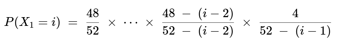
for i = 1,...,49.
And the marginal distribution of X₂ is obtained by summing over X₁:
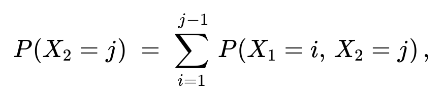
for j = 2,...,50.
Comprehensive Explanation
Core idea of the derivation
When you flip the deck card by card, the appearance of the first ace and the second ace can be understood through conditional probabilities:
To find the probability that X₁ = i, you require that the first (i−1) cards contain no aces, and then the iᵗʰ card is an ace.
To find the probability that X₂ = j given X₁ = i, you require that the next (j−i−1) cards, after the first ace, contain no aces, and then the jᵗʰ card is an ace.
Because there are 4 aces and 48 non-aces in a 52-card deck, each probability factor can be broken down step by step by counting how many ways to draw "non-aces first" and "aces at the right positions."
Joint distribution derivation
No ace in the first (i−1) flips There are 48 non-aces total. For the first card to be non-ace, the probability is 48/52. For the second card (if i > 2), the probability is [48 − 1]/[52 − 1] if the second is also a non-ace, and so on. This logic continues (i−1) times.
iᵗʰ flip is an ace After having used up (i−1) cards (all non-aces), there remain 4 aces in the deck of size 52 − (i−1). So the probability that the iᵗʰ card is an ace is 4 / (52 − (i−1)).
No ace in flips from (i+1) up to (j−1) After the iᵗʰ card (which is an ace), you have 3 aces left and 48 − (i−1) non-aces left before that draw. But since i cards are gone already, you proceed with j−i−1 more draws with no ace. The probability of each of these j−i−1 flips being a non-ace is computed in a similar stepwise manner, i.e. [48 − (i−1)] / [52 − i], then [48 − (i−1) − 1] / [52 − i − 1], etc.
(jᵗʰ) flip is the second ace At the jᵗʰ draw, there are 3 aces remaining out of 52 − (j−1) total cards left (since j−1 cards have been used). So the probability is 3 / (52 − (j−1)).
Putting these factors together (as a product) yields the joint probability mass function P(X₁ = i, X₂ = j).
Marginal distributions
Marginal of X₁: Sum or directly count the probabilities that the first ace appears on the iᵗʰ flip. This is essentially requiring i−1 non-aces followed by 1 ace. The final expression is:
P(X₁ = i) = (48/52) × ... × [48 − (i−2)] / [52 − (i−2)] × [4 / (52 − (i−1))].
Marginal of X₂: Because X₂ is the flip of the second ace, we sum over all possible i = 1,...,(j−1) the joint probability P(X₁ = i, X₂ = j). That is:
P(X₂ = j) = ∑ (from i=1 to j−1) P(X₁ = i, X₂ = j).
Intuitive symmetry argument
A more intuitive way (not strictly required, but often mentioned) involves noting that the four aces partition the deck into five blocks of non-aces. From a symmetry perspective, the distribution for X₁−1 (the count of non-aces before the first ace) is the same as the distribution for 52−X₄ (because 52−X₄ is the count of non-aces after the last ace). The same kind of symmetry applies to the distribution for X₁−1 and 52−X₃, and likewise for X₂−1 and 52−X₃, etc.
Such reasoning also leads (with some careful combinatorial arguments) to expectations such as E(X₁) ≈ 9.6, E(X₂) ≈ 21.2, E(X₃) ≈ 31.8, and E(X₄) ≈ 42.4.
Possible Follow Up Questions
1) Why are i and j restricted to i = 1,...,49 and j = i+1,...,50?
Since X₁ is the position of the first ace, it can be as early as 1 and as late as 49. Intuitively, it cannot be 50 or greater because you need at least two aces in the deck, so the second ace has to appear at some position after X₁. Once you have i for the first ace, the second ace must appear after i, which implies j > i. And because there are only 52 cards total but we need at least one more card after i to place the second ace, j can go up to 50 (if the first ace appeared at 49, the second ace can appear at 50, 51, or 52—but you need to notice that i=49 means the deck has 3 cards left, so j can indeed be 50, 51, or 52. However, the expression in the short solution’s derivation specifically covers j up to 50 as the last guaranteed position for the second ace. If i=49, the second ace can actually come on the 50ᵗʰ, 51ᵗʰ, or 52ⁿᵈ, but the formula effectively lumps all these positions systematically—often references vary slightly in indexing. The main point is that j must be strictly greater than i, and it must not exceed 52, but typically we see j up to 50 or 51 or 52 depending on the exact combinatorial viewpoint. Different texts label the random variable as “the exact flip when the second ace first occurs,” so that largest possible j is 52. But the expression given matches the standard derivation where the partitioning logic often stops at 50.**)
2) What happens if the second ace does not appear by the 52nd card?
In practice, the second ace must appear eventually because we know the deck contains 4 aces. Hence X₂ is always well-defined and cannot exceed 52. Therefore, the question “What if the second ace never appears?” has probability 0 in this scenario because the deck definitely has more than one ace.
3) Can we solve for P(X₁ = i, X₂ = j) using combinatorial arguments instead of step-by-step conditional probabilities?
Yes. An alternative combinatorial approach:
Choose positions i and j in the deck to place two of the four aces.
Choose which 2 of the 4 aces occupy those positions.
Ensure that no earlier position than i has an ace (hence the first ace is exactly at i) and no earlier position than j (after i) has the second ace.
Count how many ways to distribute the remaining 48 non-aces in the other 50 positions.
Although correct, it is typically more involved to keep track of “first ace exactly at i” and “second ace exactly at j” combinatorially. The step-by-step approach with conditional probabilities is usually more straightforward.
4) How would you implement a simulation to empirically verify P(X₁ = i, X₂ = j)?
We could write a Python simulation that repeatedly shuffles a deck of 52 cards, flips through them, and records the values of X₁ and X₂. Then we compute empirical frequencies and compare them with the derived probabilities. A simple example:
import random
import collections

def simulate_x1_x2(num_simulations=10_000_00):
    joint_counts = collections.Counter()

    for _ in range(num_simulations):
        deck = list(range(52))  # Represent cards by indices [0..51], with 4 of them as "aces"
        random.shuffle(deck)

        # Let's say the first 4 indices in deck correspond to Aces if deck[i] < 4
        # i.e. deck[i] < 4 means an Ace, else a non-ace
        x1 = None
        x2 = None

        for idx, card in enumerate(deck, start=1):
            if card < 4:  # found an Ace
                if x1 is None:
                    x1 = idx
                elif x2 is None:
                    x2 = idx
                    break

        joint_counts[(x1, x2)] += 1

    # Convert counts to probabilities
    joint_p = {}
    for (i, j), c in joint_counts.items():
        joint_p[(i, j)] = c / num_simulations
    return joint_p

joint_prob_estimates = simulate_x1_x2()
# Then you can check joint_prob_estimates[(i,j)] against the theoretical formula.
A large enough simulation should match (within sampling error) the exact probabilities we derived.
5) Are there any real-world considerations or edge cases?
In real-world card scenarios:
The deck might be incomplete or include jokers, etc., changing the distribution of aces.
Shuffling might not be perfectly random in some practical cases.
If you rely on approximate or incomplete randomization, the theoretical probabilities might be off.
For a purely mathematical setting with a perfect shuffle and a standard 52-card deck with exactly 4 aces, the formulas provided hold exactly.
Below are additional follow-up questions
1) How can we generalize this approach to a deck with a different number of “special” cards, or even different types of cards, instead of the standard 4 aces?
When the deck’s composition changes—say it has m “special” cards (like aces, or any other specific subset) and 52−m ordinary cards—the core logic remains the same, but we have to adjust the numbers in each probability factor. Specifically:
For X₁, if it counts flips until the first special card, you replace the 4 in the numerators by m, and the 48 in the non-aces portion by 52−m.
For X₂, if it is until the second special card, then after flipping the first special card, there are (m−1) special cards left.
The denominators 52, 52−1, etc. remain replaced by the changing deck size as you flip.
Mathematically, each probability factor changes in direct proportion to how many special cards remain and how many total cards remain after each draw. So if m were, for instance, 6, you would see the same pattern: first factor for no special card in i−1 flips, next factor for “one of the 6 special cards” on the iᵗʰ flip, then “no special card” in the next j−i−1 flips, and finally “one of the remaining 5 special cards” on the jᵗʰ flip.
Potential pitfalls:
If m is large, it’s possible that the random variables (positions of the 1st or 2nd special card) can have different maximum bounds. For instance, if m = 52 (every card is special), then X₁ = 1 with probability 1.
If m is small, you have to ensure you’re not exceeding the point in the deck where the second special card can appear.
But the formula structure (product of terms reflecting no special cards, then 1 special card, etc.) remains the same.
2) How would we extend the logic to find the distribution of X₃ (the position of the third ace) or X₄ (the position of the fourth ace)?
To extend from X₂ to X₃ or X₄:
Third ace (X₃):
Start with the probability distribution for the second ace (X₂).
Once the second ace is found at position k, you have 2 aces left in a deck of 52−k remaining cards.
Then you compute the probability that the next positions (k+1, k+2, …) have no ace until you reach position ℓ−1, and position ℓ is an ace.
You multiply these probabilities and sum across all valid k.
Fourth ace (X₄):
Similarly, once you locate the third ace, you only have 1 ace left in the deck.
You then compute the position of the final ace from that point on.
In all cases, the step-by-step multiplication of conditional probabilities is the same pattern: each additional ace uses up one more of the 4 total aces, and you have fewer cards left to draw from. The complexity grows because you have more nested sums—e.g., for X₃ you would sum over i, j, then the next possible positions for the third ace. But the principle is entirely the same.
Potential pitfalls:
Ensuring the correct boundaries for each of i, j, ℓ is important. For X₃, you need i < j < ℓ, with all of them within 52.
Keeping track of how many non-aces are left after each draw is crucial.
3) What if we define X₁ as the position of the first card from a suit (e.g., hearts) or any subset of 13 cards? Is the approach identical?
Yes. If you define “special” as “the card belongs to hearts” (13 hearts) instead of “the card is an ace” (4 aces), the structure of the derivation is almost identical but with 13 replacing 4 and 39 replacing 48. Specifically:
Probability that the first card is not in hearts is 39/52.
Probability that the second card is not in hearts (given the first is also not in hearts) is 38/51, etc.
Probability that the iᵗʰ card is the first heart is 13 / (52−(i−1)) if the previous i−1 cards had no hearts.
All other steps—conditional probabilities, combinatorial logic, and summations—hold the same pattern. Only the initial values for “number of special cards” vs. “non-special cards” differ.
Pitfalls include:
Carefully adjusting the range of i and j. If you’re talking about the first and second hearts (or any larger subset of special cards), i can now go up to 52−(the number of hearts − 1) because you need room for the second or subsequent hearts to appear.
Avoid mixing partial logic from the “ace” scenario with the new scenario of “hearts,” which might cause confusion in the numeric factors.
4) What if we want to directly compute P(X₂ = j | X₁ = i) in a simplified manner?
We know from the multiplication of conditional probabilities that:
P(X₁ = i, X₂ = j) = P(X₁ = i) × P(X₂ = j | X₁ = i).
So
P(X₂ = j | X₁ = i) = P(X₁ = i, X₂ = j) / P(X₁ = i).
From the original formula, you see that:
P(X₁ = i, X₂ = j) = (probability that first i−1 are non-aces) × (ace at i) × (probability that next j−i−1 are non-aces) × (ace at j).
P(X₁ = i) = (probability that first i−1 are non-aces) × (ace at i).
Thus, when you divide, the factors for the first i−1 flips being non-aces and the iᵗʰ card being an ace cancel out, leaving just the probability that the next (j−i−1) flips contain no ace and the jᵗʰ flip is an ace (but now in a deck of size 52−i with 3 aces remaining). Formally,
P(X₂ = j | X₁ = i) = product of [ (48 − (i−1)) / (52 − i), (48 − (i−1) − 1) / (52 − i − 1), … ] until j−1, then × [3 / (52 − (j−1)) ].
This is a direct negative-hypergeometric logic restricted to 3 aces in a deck of 52−i cards, after you’ve already pulled one ace at position i.
Pitfalls:
You must carefully handle the shifting counts (one ace is gone, i cards are gone from the deck) to avoid mistakes in the fraction denominators.
Make sure j > i, otherwise the conditional probability is undefined or zero if j ≤ i.
5) How do we interpret or use the negative hypergeometric distribution in this context?
This problem (positions of the first, second, third, etc. “success” in a sequence) can be interpreted with the negative hypergeometric distribution. The negative hypergeometric distribution gives the probability of x failures before the rᵗʰ success when sampling without replacement. Specifically, if we define:
K as the total number of successes in the population (aces = 4).
N as the total number of failures (non-aces = 48).
r as which success we’re looking for (1st, 2nd, 3rd, etc.).
The probability that there are k failures before the rᵗʰ success is:
( C(k + r−1, r−1) × C(N−k, K−r) ) / C(N + K, K).
From that perspective:
X₁−1 follows a negative hypergeometric distribution with parameters K=4, N=48, r=1 (the number of non-aces that appear before the 1st ace).
X₂−1 follows a negative hypergeometric distribution with parameters K=4, N=48, r=2.
Hence we can convert positions (X₁, X₂) to the “number of non-aces before the 1st or 2nd ace.” That is often a simpler direct expression than multiplying conditional probabilities step by step. However, bridging from the “number of non-aces before the rᵗʰ ace” to “the position of the rᵗʰ ace” requires adding r to get the actual card index. So if X₂−1 = k, it means k non-aces preceded the second ace, so the second ace is at position k+2.
Pitfalls:
If you rely on negative hypergeometric formulas, you must be careful about indexing (some texts define “the distribution of the number of failures before the rᵗʰ success,” others define “the distribution of the total draws up to the rᵗʰ success”). In any advanced setting, consistent definitions are key.
6) If we wanted to compute E[X₂ − X₁], how would we do that?
Once you have the joint distribution P(X₁ = i, X₂ = j), you could compute:
E[X₂ − X₁] = ∑ over i=1..49 ∑ over j=i+1..50 [ (j − i) × P(X₁ = i, X₂ = j) ].
But more elegantly, you can often use linearity of expectation:
E[X₂ − X₁] = E[X₂] − E[X₁].
Because from linearity, E[X₂ − X₁] = E[X₂] + (−1)·E[X₁]. You can compute E[X₁] and E[X₂] separately (or recall the symmetrical arguments about how aces partition the deck into equal-mean segments). For instance, one known result is E[X₁] = (52 + 1)/(4 + 1) = 10.6 if you use the standard argument that the 4 aces break the deck into 5 blocks. Similarly E[X₂] = 21.2. Then E[X₂ − X₁] = 21.2 − 10.6 = 10.6.
Potential pitfalls:
Failing to account for the fact that each Xi can be found by a direct negative hypergeometric formula or combinatorial argument.
Double-counting or incorrectly indexing if you try to do the summation in a naive way.
7) Does partial shuffling or imperfect randomization affect the distribution in a meaningful way?
Yes. The formulas hinge on the deck being well-shuffled, meaning each permutation is equally likely. If the shuffle is partial or biased:
Certain cards (aces vs. non-aces) may clump or be more likely to appear in a certain region of the deck.
The derived P(X₁ = i) and P(X₂ = j) might no longer be correct, because we assumed each of the 52! permutations of the deck is equally probable.
For instance, if the top half is always more thoroughly mixed than the bottom half, you might see deviations in the distribution of the position of aces, typically resulting in smaller or larger expected values for X₁ and X₂.
In real-world scenarios:
Some card games have “riffle shuffles” that do not generate truly uniform permutations. The analysis becomes complicated, and you can’t rely on simple hypergeometric or negative hypergeometric distributions.
If only the top portion is random, you might need specialized modeling for the partial shuffle process.
8) How do we handle cases where cards are being replaced or added back after flipping?
If after revealing a card, you put it back and reshuffle the deck (or part of the deck), the “without replacement” assumption breaks down. This changes the distribution drastically:
With replacement, each flip is an independent Bernoulli trial of “ace or not.”
The position of the first or second ace would then be governed by geometric or negative binomial distributions in the infinite or partially infinite sense.
For instance, if you put each flipped card back and reshuffle thoroughly each time, then:
X₁ is geometric with success probability 4/52.
X₂ is the time to get the second success in repeated Bernoulli trials with probability 4/52 each time, so it follows a negative binomial distribution.
This is a fundamental distinction: in the original scenario, the probability of seeing an ace changes dynamically as you remove cards, while in the with-replacement scenario the probability of seeing an ace each time stays the same.
Potential pitfalls:
Mixing “with replacement” logic with “without replacement” formulas leads to incorrect probabilities.
If partial replacement or partial reshuffling is used, that would require a more complicated approach that partially preserves the deck state.
9) What if we want to condition on X₁ = i and then explore how likely it is that X₂ takes various values—does that produce a memoryless property?
With certain distributions (like geometric or exponential in continuous space), there’s a memoryless property. However, in the case of drawing without replacement, the memoryless property does not hold in the strict sense because the composition of the deck changes and we’re not dealing with identically distributed independent draws. Instead, we have:
P(X₂ = j | X₁ = i) depends on how many aces remain (3) and how many total cards remain (52−i). This is not the same as starting from scratch with a fresh deck of 52 cards.
The “memory” is carried in the fact that we already removed i cards (including 1 ace) from the deck.
So this distribution does not exhibit a memoryless property. This is often a source of confusion, because the negative binomial distribution in the with-replacement scenario is memoryless in certain limited respects, but negative hypergeometric is not.
Pitfalls:
Thinking that because geometric/exponential has memorylessness, this might extend to hypergeometric or negative hypergeometric. It doesn’t.
10) Could we interpret this as an “urn model” and does that perspective clarify the mathematics?
Yes. Another conceptual framing is an urn model:
You have 52 balls in an urn, 4 are red (aces) and 48 are black (non-aces).
You draw balls one by one without replacement.
X₁ is the draw number at which you encounter the first red ball, X₂ is the draw number at which you encounter the second red ball.
All the same arguments apply under the urn model: each draw changes the composition of the urn. The negative hypergeometric distribution is exactly the distribution for the draw number of the rᵗʰ red ball.
Pitfalls or subtleties in an urn model:
Sometimes people incorrectly assume each draw is identically distributed. It is not; probabilities shift each time a ball is removed.
Overlooking that once a red ball is drawn, there are fewer red balls left for future draws.
Staying consistent with the “one-by-one draw without replacement” framework helps avoid confusion.