
ML Interview Q Series: Joint PMF for Sequentially Dependent Binomial Random Variables

Browse all the Probability Interview Questions here.
11E-1. (b) You have two fair coins. The first coin is tossed five times. Let the random variable X be the number of heads showing up in these five tosses. The second coin is then tossed X times. Let Y be the number of heads showing up in those X tosses. What is the joint probability mass function of X and Y? What is E(X + Y)?
Short Compact solution
The joint probability mass function is:
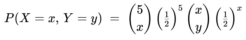
for 0 <= x <= 5 and 0 <= y <= x.
Using the relation E(X + Y) = sum over x from 0 to 5 of sum over y from 0 to x of (x + y) * P(X = x, Y = y), one finds:
E(X + Y) = 2.5 + 1.25 = 3.75.
Comprehensive Explanation
Underlying Setup
We have two fair coins:
Coin 1 is tossed 5 times.
Let X be the number of heads observed among these 5 tosses.
Because Coin 1 is fair, each toss has probability 1/2 of being heads.
The distribution of X is binomial with parameters n=5 and p=1/2. This implies that P(X = x) = (5 choose x) (1/2)^5 for x=0..5.
Coin 2 is tossed X times.
Let Y be the number of heads observed among those X tosses of Coin 2.
Coin 2 is also fair, so each toss again has probability 1/2 of being heads, independently of all other tosses.
Conditional on X, Y is binomial with parameters n=X and p=1/2.
Derivation of the Joint PMF
To find the joint pmf P(X = x, Y = y), we first note:
The probability that the first coin shows x heads in 5 tosses is (5 choose x)(1/2)^5.
Given X = x, the probability that the second coin shows y heads in x tosses is (x choose y)(1/2)^x.
Since the outcome of the second coin depends on X but is otherwise independent, we multiply these probabilities:
$$P(X = x, , Y = y)
;=; \bigl[\binom{5}{x},\bigl(\tfrac12\bigr)^5 \bigr] ;\times; \bigl[\binom{x}{y},\bigl(\tfrac12\bigr)^x \bigr]$$
with valid values 0 <= x <= 5 and 0 <= y <= x.
Expected Value E(X + Y)
We want to find E(X + Y). One efficient way is to use the law of total expectation and the known relationships for binomial random variables:
E(X) for X ~ Binomial(5, 1/2) is 5 * (1/2) = 2.5.
For Y conditional on X = x, we have Y ~ Binomial(x, 1/2). Hence E(Y | X = x) = x/2.
Therefore, E(Y) = E( E(Y | X) ) = E( X/2 ) = (1/2)*E(X) = 1.25.
Summing them up:
E(X + Y) = E(X) + E(Y) = 2.5 + 1.25 = 3.75.
This agrees perfectly with the explicit summation approach.
Why the PMF Works Only for 0 <= y <= x
It is crucial that Y can never exceed the number of tosses X; hence the support for Y is y = 0..x. If x = 0 (i.e., we got no heads on the first coin's five tosses), the second coin is not tossed at all, so Y must be 0 in that case, which is consistent with (0 choose 0)(1/2)^0 = 1.
Practical Interpretation
On average, you expect 2.5 heads from the first batch of 5 tosses (that is your variable X).
Then you toss the second coin X times. If X is 2.5 on average, you expect half of those to be heads, giving E(Y) = 1.25.
Thus in total, E(X + Y) = 3.75 heads across the entire process.
Potential Follow-Up Questions
How would we generalize this if the coins were biased with different probabilities?
If the first coin has probability p (instead of 1/2) of landing heads, then X ~ Binomial(5, p). So P(X = x) = (5 choose x) p^x (1-p)^(5-x). If the second coin has probability q of landing heads, then, given X = x, Y ~ Binomial(x, q). So P(Y = y | X = x) = (x choose y) q^y (1-q)^(x-y). The joint pmf then becomes:
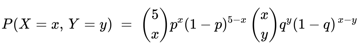
for 0 <= x <= 5 and 0 <= y <= x.
The expectation E(X + Y) can be found using E(X + Y) = E(X) + E(Y) = 5p + E(X)q. Since E(X) = 5p, we have E(Y) = E(X)q = 5pq, so:
E(X + Y) = 5p + 5pq = 5p(1 + q).
Can you derive E(X + Y) directly using moment generating functions or probability generating functions?
Yes, one can use moment generating functions (MGFs) or probability generating functions (PGFs). For instance, the PGF of a Binomial(n, p) random variable X is G_X(t) = (1 - p + pt)^n. Then, if Y | X = x ~ Binomial(x, q), its conditional PGF is G_{Y|X=x}(t) = (1 - q + qt)^x. One can then compute:
E(X + Y) = d/dt [ G_{X,Y}(t) ] at t=1,
though typically the law of total expectation is a simpler route in this problem.
Edge Cases and Special Situations
If X = 0, no tosses occur for the second coin, forcing Y = 0 with probability 1 in that scenario.
If X = 5, then the second coin is tossed 5 times, so Y can go all the way up to 5.
The event X = 5 has probability (1/2)^5, while for Y = 5 given X=5 is also (1/2)^5.
Python Code Snippet to Simulate
Below is a quick Python snippet demonstrating how one might empirically estimate E(X+Y) via simulation:
import numpy as np

num_trials = 10_000_00
results = []

for _ in range(num_trials):
    # First coin tossed 5 times
    x = np.sum(np.random.rand(5) < 0.5)

    # Second coin tossed x times
    y = np.sum(np.random.rand(x) < 0.5)

    results.append(x + y)

empirical_mean = np.mean(results)
print("Empirical E(X+Y) =", empirical_mean)
Running this code repeatedly should give an empirical mean close to 3.75, confirming our theoretical calculation.
Below are additional follow-up questions
1) How would you derive the distribution of X+Y directly without conditioning on X?
To find the distribution of X+Y, we note:
X ~ Binomial(5, 0.5).
Conditioned on X=x, Y ~ Binomial(x, 0.5).
One might try to convolve these distributions, but it is more subtle than a direct convolution of two binomials, because Y's number of trials depends on X. A standard approach is to use:
X+Y = X + (sum of Y_i), where Y_i indicates each head from the second set of tosses. But each Y_i only exists if X >= i. Another strategy uses probability generating functions or moment generating functions, but it becomes cumbersome.
Pitfall: Careless attempts might treat X and Y as independent binomials or incorrectly do a straightforward convolution, ignoring that Y’s parameter depends on X. This leads to an incorrect distribution.
Edge Case: Notice that X+Y cannot exceed 10 if X=5 and Y=5. Also, X+Y can be as low as 0 (if X=0 and hence Y=0). Any attempt to compute P(X+Y = k) must account for all valid values of x and y such that x+y=k and y <= x.
2) If we replace the second coin with a die roll to decide Y’s number of successes, how does that change the approach?
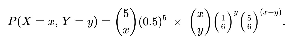
Imagine we still have X ~ Binomial(5, 0.5), but then we do something more complicated for Y. For instance, if we roll a 6-sided die X times, and define Y to be the count of outcomes that equal 6 (probability 1/6 each roll). Mathematically:
X is still Binomial(5, 0.5).
Given X=x, Y ~ Binomial(x, 1/6).
The structure remains a two-stage binomial, but with a different probability for the second stage. The joint pmf generalizes readily:
Pitfall: Failing to recognize that Y’s success probability differs from X’s success probability can lead to confusion or using the wrong formula.
Edge Case: If X=0, there are no die rolls, so Y=0 with probability 1. This is consistent with binomial(x=0, p=1/6).
3) What happens if the second stage is not binomial at all, but rather uses a non-i.i.d. process for Y?
Suppose that instead of tossing a fair coin X times independently, you have a correlated or different distribution for Y. For example, each toss might depend on the previous toss or might come from a more exotic distribution (like a geometric or negative binomial sampling process). Then:
X is still Binomial(5, 0.5).
Given X=x, Y might have some distribution more complicated than Binomial(x, 0.5).
The formula for P(X=x, Y=y) would be:
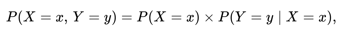
but now P(Y=y | X=x) is not just a simple binomial formula. It depends on the chosen distribution.
Pitfall: Confusing the memoryless property of a geometric distribution with that of a binomial distribution can lead to incorrect computations.
Edge Case: If the second stage’s random process fails to produce a well-defined maximum number of successes, you can have an unbounded Y even if X=5. This obviously wouldn’t align with the standard binomial setup and demands a re-examination of how the second stage is defined.
4) How would you handle the variance calculation of X+Y?
The law of total variance is typically used. We know:
Var(X+Y) = E[ Var(X+Y | X) ] + Var( E[X+Y | X] ).
Because E(X+Y | X=x) = x + x/2 = 1.5x, and Var(X+Y | X=x) = Var(X) + Var(Y|X=x) only if X and Y|X are independent. However, we must be careful because X and Y share a dependence through x. The correct approach is:
E(Y | X=x) = x/2, Var(Y | X=x) = x(1/2)(1 - 1/2) = x/4.
Then E(X+Y | X=x) = x + x/2 = 1.5x, Var(X+Y | X=x) = Var(X=constant given x) + Var(Y|X=x). But X is known in the conditional, so Var(X=constant) = 0. So Var(X+Y | X=x) = x/4.
Hence:
E[Var(X+Y | X)] = E(x/4) = (1/4)E(x) = (1/4)*2.5 = 0.625.
Var( E[X+Y | X] ) = Var(1.5X) = (1.5)^2 Var(X). Since Var(X)=np(1-p)=5*(1/2)(1/2)=51/4=1.25, that part is (1.5)^2 * 1.25 = 2.25 * 1.25 = 2.8125.
So Var(X+Y) = 0.625 + 2.8125 = 3.4375.
Pitfall: A common mistake is to assume X and Y are independent and do Var(X+Y) = Var(X)+Var(Y), ignoring Y’s dependence on X.
Edge Case: If p=0 for the first coin (always tails), then X=0 deterministically, so Y=0 always, thus Var(X+Y)=0. Such boundary conditions are a good sanity check.
5) How would you interpret X and Y if this were a real-world scenario, such as software A/B testing?
Imagine X is the count of successes (e.g., user sign-ups) out of 5 randomly chosen visitors in an A/B test. Then you choose exactly X new visitors to show the software, and measure Y as the count of sign-ups among those X. The joint distribution formalism is the same, but the interpretation shifts to a real-world funnel problem.
Potential complexities:
The second group might have different behavior from the first, or might overlap with the first group, violating independence assumptions.
The success probability might vary with time or user segment, invalidating the binomial assumption.
Pitfall: Real-world data often shows correlation or changing probabilities across cohorts. That breaks the tidy binomial assumption and might require a Beta-Binomial or hierarchical approach.
Edge Case: If no one signs up in the first wave (X=0), you might not even run the second wave. This can lead to missing data or alternative decisions in practical settings.
6) How might you extend this to a Bayesian setting with unknown coin bias?
In a Bayesian setting, you do not assume the coin’s bias is 0.5 but instead put a prior, say Beta(α, β), on the probability p of heads. Then:
You observe X heads out of 5 from the first coin. You update the posterior for p based on that observation.
Given that updated posterior, the distribution of p influences how many times heads will appear in the next X tosses for the second coin.
The full joint distribution becomes more involved because p is no longer fixed, so you integrate over the posterior distribution of p. Symbolically:
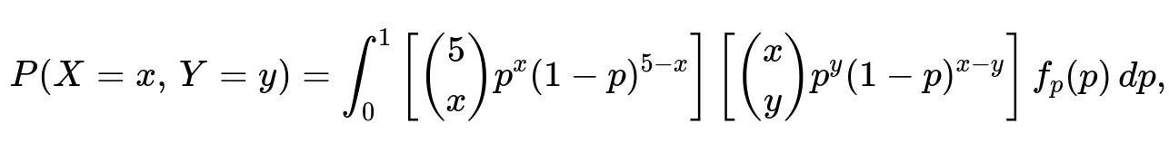
where f_{p}(p) is the prior for p. If that prior is Beta(α, β), it updates to Beta(α + x, β + 5 - x) after observing X.
Pitfall: Failing to integrate over the posterior for p leads to treating p as known, which can misrepresent parameter uncertainty.
Edge Case: If α or β is very small or large, it heavily skews the prior, possibly overshadowing the data from just 5 tosses. This can produce large differences in predictions for Y compared to a more neutral prior.
7) What if you have multiple coins with random toss counts, rather than just one coin followed by another?
Consider an experiment with n stages, where stage i’s number of tosses is determined by the result from stage i-1. Then you have a chain of random variables X_1, X_2, …, X_n, where X_1 might be binomial with parameters (5, 0.5), then X_2 is binomial with parameters (X_1, 0.5), X_3 is binomial with parameters (X_2, 0.5), and so on. Formally:
X_1 ~ Binomial(5, 0.5), X_2 | X_1 ~ Binomial(X_1, 0.5), X_3 | X_2 ~ Binomial(X_2, 0.5), ...
This structure is more involved but can be generalized using the same hierarchical approach: P(X_1, X_2, …, X_n) = P(X_1) * P(X_2|X_1) * … * P(X_n|X_{n-1}).
Pitfall: Doing naive summations or ignoring the chain dependencies can yield incorrect results. The distribution of X_n can be quite complex (a Poisson-binomial or iterated binomial form).
Edge Case: If any X_i=0, all subsequent X_j=0 for j>i. This abrupt chain termination must be carefully tracked in the distribution.
8) How does the Central Limit Theorem apply, if at all, for X+Y?
The direct CLT question arises if the number of trials (like 5 tosses for the first coin) grows. With only 5 tosses, the distribution is small and discrete. But if we let the first coin be tossed n times with probability p, then X ~ Binomial(n, p). For large n, X is approximately normal with mean np and variance np(1-p). The second stage has Y | X ~ Binomial(X, q). As n grows large, we might do a two-level approximation. Typically:
E(X) = np, Var(X) = np(1-p), E(Y | X) = qX, Var(Y | X) = q(1-q)X.
One can attempt a normal approximation to X, then approximate Y around its conditional mean. This leads to a compound distribution that can often be approximated by a normal for large n.
Pitfall: Using a normal approximation for small n=5 is inaccurate. The normal approximation is better for large sample sizes.
Edge Case: If p or q is extremely close to 0 or 1, the binomial distribution can be highly skewed, diminishing the accuracy of a normal approximation even for moderately large n.
9) How might you test if the theoretical pmf agrees with empirical data from real experiments?
You could:
Collect large amounts of (X, Y) pairs from actual experiments.
Estimate the frequency distribution of (X, Y).
Compare that empirical distribution to the theoretical pmf P(X=x, Y=y) using a chi-square goodness-of-fit test or other statistical tests.
Pitfall: If the coin tosses are not truly independent or the coin is not truly fair, you might see significant deviations.
Edge Case: If the sample size is small, the chi-square test may not be appropriate or might have low power, especially for low probabilities like X=5, Y=5. In that case, specialized small-sample tests or exact methods might be needed.
10) If an error in the setup causes the second coin to be tossed a fixed number of times, say 5, no matter what X is, how does that change the analysis?
Then Y is simply Binomial(5, 0.5), independent from X. So:
P(X = x) = (5 choose x)(0.5)^5.
P(Y = y) = (5 choose y)(0.5)^5.
The joint pmf is P(X = x, Y = y) = P(X = x)*P(Y = y), because they are independent.
Pitfall: If your code or experiment accidentally implements a fixed number of tosses in the second stage instead of X tosses, your theoretical derivations that assume Y depends on X become invalid.
Edge Case: If you discover that Y’s distribution matches a binomial(5, 0.5) exactly, it might be a clue that your experiment didn’t incorporate the dependence of the second stage on the first stage.