
ML Interview Q Series: Joint Probability and Negative Correlation Between Exclusive Outcomes in Dice Rolls
Browse all the Probability Interview Questions here.
A fair die is rolled six times. Let X be the number of times a 1 is rolled and Y be the number of times a 6 is rolled. What is the joint probability mass function of X and Y? What is the correlation coefficient of X and Y?
Short Compact solution
The joint probability mass function is
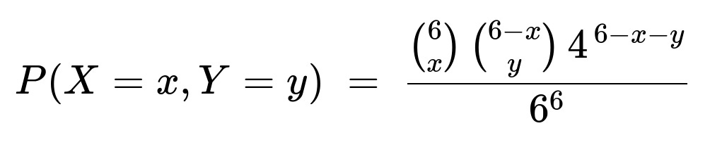
for x, y >= 0 and x + y <= 6. The correlation coefficient of X and Y is -0.2.
Comprehensive Explanation
Deriving the Joint PMF
When a fair die is rolled 6 times, each roll can land on exactly one face from 1 through 6. We define X as the number of times face 1 is rolled, and Y as the number of times face 6 is rolled. Because each roll is independent, we can think as follows:
The probability of rolling a 1 on any single trial is 1/6.
The probability of rolling a 6 on any single trial is also 1/6.
The probability of rolling any other face (2, 3, 4, or 5) on a single trial is 4/6.
We need the probability that exactly x out of the 6 rolls are 1, y out of the remaining 6 - x rolls are 6, and the rest 6 - x - y are any of the other four faces. The number of ways to choose which x rolls are 1 is "6 choose x", and then among the remaining 6 - x rolls, the number of ways to choose which y rolls are 6 is "(6 - x) choose y". The remaining 6 - x - y rolls will each be one of the 4 faces that are neither 1 nor 6.
Putting it all together:
The binomial coefficients determine the number of ways to position x occurrences of 1 and y occurrences of 6 among the 6 trials.
Each time we get a 1, the probability is 1/6.
Each time we get a 6, the probability is 1/6.
Each time we get any other face, the probability is 4/6.
Overall, we must divide by 6^6 for all possible outcomes of six rolls (each of the 6 trials can land on one of 6 faces independently).
However, a neat combinatorial approach (which also appears in many references) is to treat the “four other faces” collectively as if they are a single “combined” outcome of probability 4/6. Hence the joint pmf:
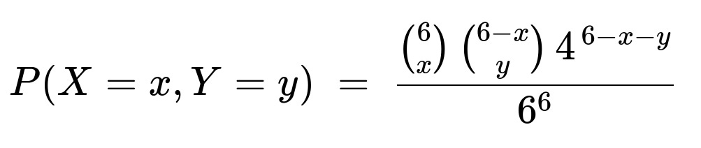
Here:
x is the count of 1's in the 6 rolls.
y is the count of 6's in the 6 rolls.
The factor (4^(6 - x - y)) arises because each of the remaining (6 - x - y) rolls can be any of the four remaining faces (2, 3, 4, or 5).
The pmf is valid only for x, y >= 0 such that x + y <= 6, because you cannot have x 1's and y 6's that together exceed 6 total rolls.
Computing the Correlation Coefficient
Mean and Variance of X and Y
Each of X and Y follows a Binomial(6, 1/6) distribution when considered individually (though they are not mutually independent). For a Binomial(n, p) random variable, the mean is n p and the variance is n p (1 - p). Thus:
E(X) = 6 * (1/6) = 1
Var(X) = 6 * (1/6) * (5/6) = 5/6
Similarly,
E(Y) = 6 * (1/6) = 1
Var(Y) = 5/6
Computing E(XY)
To see why X and Y have negative correlation, note that on a single roll, it cannot be both 1 and 6 simultaneously. One standard way to find E(XY) is to introduce indicator variables:
Let I_j = 1 if the j-th roll is a 1, and 0 otherwise.
Let L_k = 1 if the k-th roll is a 6, and 0 otherwise.
Then
X = I_1 + I_2 + ... + I_6 Y = L_1 + L_2 + ... + L_6
and
XY = (I_1 + ... + I_6)(L_1 + ... + L_6).
When you expand XY, the term I_j L_j is always 0 for any single roll j, because you cannot have a roll be both 1 and 6. Hence I_j * L_j = 0. What remains are cross terms for j != k:
XY = sum over j != k of (I_j L_k).
Since for j != k, I_j and L_k involve different rolls, they are independent and we have E(I_j L_k) = E(I_j) * E(L_k) = (1/6)(1/6) = 1/36. There are 6 * 6 = 36 total pairs (j, k), but only 36 - 6 = 30 are the pairs with j != k. Therefore,
E(XY) = 30 * (1/36) = 30/36 = 5/6.
Covariance and Correlation
The covariance between X and Y is
cov(X, Y) = E(XY) - E(X) E(Y).
We already have E(X) = 1, E(Y) = 1, and E(XY) = 5/6. Thus
cov(X, Y) = 5/6 - (1)(1) = 5/6 - 1 = -1/6.
Then the correlation coefficient is
cor(X, Y) = cov(X, Y) / sqrt(Var(X) Var(Y)).
Given Var(X) = 5/6 and Var(Y) = 5/6, we get
cor(X, Y) = (-1/6) / sqrt((5/6)(5/6)).
Simplify:
sqrt((5/6)(5/6)) = 5/6,
Hence cor(X, Y) = (-1/6) / (5/6) = (-1/6) * (6/5) = -1/5 = -0.2.
Why the Negative Correlation?
Intuitively, if you know that there were many 1’s in the 6 rolls, it becomes slightly “harder” for there also to be many 6’s, because that would require multiple rolls simultaneously to be both 1 and 6. Although each of X and Y individually has expectation 1, jointly they tend to “push each other down,” so to speak, and that is captured by a negative covariance/correlation.
Possible Follow-up Questions
1) Why are X and Y not independent?
X and Y are not independent because knowing that you already have x = 6 (i.e., all rolls were 1) makes it impossible to have y > 0. Formally, if X = x, then only 6 - x rolls remain to be anything else, including the possibility of being 6. Hence the outcome constraints couple X and Y together.
2) How can one simulate this scenario in Python?
You can simulate rolling a fair die six times many times and count occurrences of 1’s and 6’s, then estimate the joint pmf and correlation coefficient:
import random
import statistics

trials = 10_000_00  # large number of trials
counts_x = []
counts_y = []

for _ in range(trials):
    rolls = [random.randint(1, 6) for _ in range(6)]
    x_val = sum(1 for r in rolls if r == 1)
    y_val = sum(1 for r in rolls if r == 6)
    counts_x.append(x_val)
    counts_y.append(y_val)

# Empirical correlation
corr = statistics.correlation(counts_x, counts_y)
print("Empirical correlation:", corr)
We expect the result to be very close to -0.2.
3) Can you generalize this to other faces or a different number of rolls?
Yes. If you define X to be the count of face a and Y to be the count of face b in n rolls of a fair die, the same reasoning applies. The joint pmf simply changes the binomial coefficients and exponent base in a straightforward way, and the negative correlation pattern holds whenever a != b because a single roll cannot be both a and b simultaneously.
4) What if we had a loaded (non-fair) die?
For a loaded die, each face i might have probability p_i (where the sum of all p_i = 1). Then for each roll:
Probability of rolling face a is p_a.
Probability of rolling face b is p_b.
Probability of rolling neither face a nor face b is 1 - p_a - p_b.
The derivation of the joint pmf is similar, except that we would use p_a for face a, p_b for face b, and (1 - p_a - p_b) for the other faces. You can rewrite the formula for the pmf accordingly and compute means, variances, and the correlation. You would still observe negative correlation if face a and face b cannot occur on the same roll, though the exact correlation numeric value would differ from -0.2.
5) Are there any practical scenarios in machine learning or data analytics where we see a similar phenomenon?
Yes, scenarios in multi-label classification or multi-event tracking can show negative correlations when two events are mutually exclusive on any given “trial.” For example, if you are logging what category a user clicks on a page, and categories are mutually exclusive, you may find that the random variables counting how many times users click category A vs. category B in a batch of user sessions have negative correlation.
Such a negative correlation might not necessarily be strong in real data (unlike a perfectly exclusive event), but the mutual exclusivity or near-exclusivity leads to correlation coefficients less than zero.
Below are additional follow-up questions
1) What if we wanted to model the counts of three faces simultaneously (e.g., the number of times we get a 1, a 6, and a 2) instead of just two?
In many practical scenarios, you might be interested in more than two outcomes. For instance, you might define X as the count of 1’s, Y as the count of 6’s, and Z as the count of 2’s in 6 rolls. A direct extension uses the multinomial framework, where the joint pmf would involve multinomial coefficients. Specifically, for three mutually exclusive categories (faces 1, 6, and 2), if p1 = 1/6, p2 = 1/6, p3 = 1/6, and the rest p_other = 3/6, then the probability that X = x, Y = y, Z = z (and the remaining 6 - x - y - z are any of the other faces) is given by:
for x + y + z <= 6. This is an obvious generalization of the binomial approach. You could then analyze pairwise correlations among (X, Y, Z) or more advanced measures like partial correlations among the three variables. The main pitfall here is that as you track more categories simultaneously, you have to ensure your data is not too sparse (i.e., you have enough trials to estimate these joint probabilities reliably), or else your estimates of correlations might be noisy.
2) How do we handle scenarios where the total number of rolls is very large, and we want an asymptotic view of correlation?
When the number of rolls n grows large, each of the random variables X and Y (counts of particular faces) can be approximated by a binomial distribution with parameters (n, 1/6). As n → ∞, by the Law of Large Numbers, X/n converges to 1/6, and Y/n converges to 1/6. Their correlation remains negative, but the magnitude of the correlation might become more interpretable if you look at standardized counts. Indeed, the correlation formula itself,
cov(X, Y) / sqrt(var(X) * var(Y)),
does not vanish as n increases; it instead approaches a fixed limit (like -0.2 in the 6-roll case, though with a larger n you would recalculate it accordingly). A subtlety is that for large n, the distribution of X and Y gets sharper around n/6, so while the correlation might remain negative, the relative standard deviation shrinks compared to n. Practically, if X or Y is extremely small or large, numerical instabilities can occur in computing correlation in a software package, especially if the sample size is not large enough to validate a normal approximation.
3) Could there be a scenario where correlation is zero but the variables are still dependent?
Absolutely. Correlation measures only the linear relationship between two variables. If the variables are related in a more complex, non-linear way, their correlation can be zero (or close to zero) yet they remain dependent. In a dice-roll context, a contrived example might be if you define a random variable that is 1 when X is in {0,1,2,3} and 0 otherwise, and compare it to another carefully constructed function of Y. Even though these could be related via a non-linear rule, the computed Pearson correlation might be zero. The pitfall is assuming that zero correlation implies independence, which is not always true. You would need more advanced dependency metrics (e.g., mutual information) to capture such relationships.
4) If we let X be the number of times we roll a 1 or a 2 (instead of just 1), and Y be the number of times we roll a 3 or a 6, would we still see a negative correlation?
Yes, but it might differ in magnitude. As long as each die roll belongs exclusively to either the “(1 or 2)” event or the “(3 or 6)” event (plus any other outcomes), there is an inherent exclusion in a single roll, which can induce a negative correlation. The sign of correlation is still typically negative because more occurrences of “1 or 2” leaves fewer opportunities for “3 or 6” on a fixed number of rolls. However, the exact correlation value depends on the respective probabilities: p(1 or 2) = 2/6 = 1/3, p(3 or 6) = 2/6 = 1/3, so the combinatorial structure is somewhat altered, as is the probability that each event occurs on a single roll. Be aware that the correlation magnitude might change because the means and variances of X and Y shift when we group multiple faces together.
5) What if we consider a continuous analog of this problem, such as distributing a certain number of events into categories over time?
In continuous-time or continuous-event settings (e.g., Poisson processes), each event can go into exactly one of several exclusive “bins” or categories. If we define X as the count of events in category 1 over a fixed interval, and Y as the count in category 2 over that same interval, then the correlation could again be negative if the categories are exclusive. In fact, for a multinomial Poisson process, you have a partitioning of events into multiple sub-processes, and often the sub-process counts exhibit negative correlations because an event’s occurrence in one sub-process excludes it from another. A subtlety is that, in continuous-time processes, we also have to consider rates, concurrency, and whether the process is truly Poisson or has more complex dependence. The main pitfall is that the discrete dice-rolling logic does not translate directly to a continuous environment if events can overlap, so checking assumptions is crucial.
6) Could partial correlations introduce a different sign of relationship if we condition on a third variable?
Partial correlation measures the relationship between two variables while controlling for the effect of a third (or multiple) variable(s). Suppose you define W as the total number of times you roll either a 1 or a 6 combined. You could then compute the partial correlation between X and Y given W. Because X + Y = W, that partial correlation might behave quite differently. In fact, if X and Y sum to a constant W, that implies X = W - Y, and we might see that controlling for W essentially forces a perfect negative linear relationship between X and Y, so the partial correlation could be exactly -1. The pitfall is failing to realize that conditioning on a variable that is perfectly collinear (like X + Y) can drastically alter correlation measures and produce boundary effects (e.g., ±1).
7) How do we reconcile the fact that X and Y can never exceed 6 in total, yet we talk about standard correlation like it’s an unbounded linear measure?
Pearson’s correlation is typically derived for variables that can, in principle, take on a wide range of values. However, X and Y here are bounded by 0 and 6, creating a finite, discrete sample space. The correlation measure is still valid, but one has to remember that the random variables are discrete with limited support. In some circumstances, a measure like Spearman’s rank correlation or Kendall’s tau might give additional insights into monotonic relationships. A pitfall is overinterpreting a correlation coefficient in a bounded discrete scenario the same way you would in an unbounded continuous scenario. For instance, a correlation of -0.2 might have a different “strength” interpretation in a discrete, small-range setting than in large continuous data.
8) If you label each die roll outcome from 1 to 6 and think of that as categorical data, what other statistical tests or measures (besides correlation) might you use to assess relationships?
With categorical data, common analyses include chi-square tests of independence or mutual information. For example, if you define two random variables that each summarize the outcomes of multiple rolls, you can create a contingency table and run a chi-square test to see if the joint distribution deviates from what independence would predict. Mutual information gives a more general measure of the amount of uncertainty reduced in one variable by knowledge of the other. These approaches may be more suitable than correlation if the relationship is not strictly linear. The pitfall is applying Pearson correlation alone to purely categorical settings and concluding independence or dependence without verifying that the linear relationship concept is even appropriate.
9) What happens if we only roll the die twice or three times? Does the correlation still make sense?
Even with only two or three rolls, you can still define X as the count of 1’s and Y as the count of 6’s, and compute the covariance and correlation in a theoretical sense. The pmf will be simpler, and you could compute expectations directly. For example, if there are only two rolls, then X and Y each take values in {0, 1, 2}, but obviously they can’t both be 2 at the same time. You would still see a negative correlation, though the exact numeric value would differ from the six-roll scenario. However, interpreting correlation in such a small trial might be less meaningful because the variance is extremely small. A pitfall arises if you try to do an empirical estimate of correlation from minimal data—small-sample artifacts can be large, so statistical estimates of correlation might not be stable.
10) How could generating functions or probability generating functions help in deriving or confirming these correlations?
A probability generating function (PGF) for a discrete random variable X is E(t^X). If you define G(t, s) = E(t^X s^Y), you get a two-variable generating function capturing the joint distribution of X and Y. From G(t, s), you can differentiate with respect to t and s at t=1, s=1 to get moments such as E(X), E(Y), and E(XY). Specifically:
E(X) = partial derivative of G(t, s) wrt t evaluated at t=1, s=1.
E(Y) = partial derivative of G(t, s) wrt s evaluated at t=1, s=1.
E(XY) = partial mixed derivative wrt t and s evaluated at t=1, s=1.
This provides a systematic approach to confirm the covariance or correlation. The pitfall is that generating functions can become cumbersome for large n or multiple categories, so you have to keep careful track of partial derivatives, but it’s a powerful tool for proofs and symbolic manipulations.