
ML Interview Q Series: Joint Probability Mass Function for Highest & Second-Highest Scores in d Dice Rolls

Browse all the Probability Interview Questions here.
11E-5. You simultaneously roll (d) fair dice. Let the random variable (X) be the outcome of the highest scoring die and (Y) be the outcome of the second-highest scoring die, with the convention that (Y = X) if two or more dice show the highest score. What is the joint probability mass function of (X) and (Y)?
Short Compact solution
For each integer (i) from 1 to 6, the probability that both the highest and second-highest scores equal (i) is

For (i > j), the probability that the highest score is (i) and the second-highest score is (j) is
Comprehensive Explanation
Overview of the Problem
We roll (d) fair six-sided dice (each die takes values 1 to 6 with probability 1/6). We define:
(X) as the maximum (highest) face value among the (d) dice.
(Y) as the second-highest face value, with the convention that (Y) equals (X) if there are at least two dice showing the maximum value.
Thus, the possible pairs ((X,Y)) satisfy (1 \le Y \le X \le 6). When (X = i) and (Y = i), it means at least two dice show the value (i), and all other dice show values strictly less than (i). When (X = i) and (Y = j) with (i > j), it means that:
At least one die shows (i).
No die shows a value greater than (i).
At least one die shows (j), and all other dice show values (\le j).
Among those (\le j) dice, nobody reaches (j+1, j+2,\dots, i-1).
And importantly, we do not have two or more dice at the highest value (i); otherwise (Y) would have become (i).
Case 1: (P(X=i, Y=i))
The event ({X = i, Y = i}) means:
There are at least two dice showing the value (i).
All other dice show values strictly less than (i).
One way to count this is:
Choose (r) dice (where (r \ge 2)) to show the value (i). There are (\binom{d}{r}) ways to choose which (r) dice show (i).
Each of those (r) dice has probability ((1/6)) of showing (i).
Each of the remaining (d-r) dice must show a value from ({1, 2,\dots, i-1}), so each has probability (\frac{i-1}{6}).
Hence the sum
[ \huge \sum_{r=2}^{d} \binom{d}{r}\left(\frac{1}{6}\right)^r\left(\frac{i - 1}{6}\right)^{d-r}. ]
Through binomial expansions and algebra, that sum simplifies to
[ \huge \frac{i^{d} - (i-1)^{d} - d,(i-1)^{d-1}}{6^{d}}. ]
The high-level idea behind this closed-form expression is to consider:
(i^{d}) counts all ways dice can take values in ({1,\dots,i}) with no restriction (i.e., the number of length-(d) strings from an alphabet of size (i)).
((i-1)^{d}) counts all ways if dice are restricted to values (\le i-1).
Subtracting these helps isolate those configurations that reach at least one die with value (i).
The extra term (-,d,(i-1)^{d-1}) removes the cases in which exactly one die is (i), because in that scenario we would have (Y< i), contradicting (Y=i). Hence we exclude that single-(i) scenario by accounting for the ways exactly one die is (i) and the rest are (\le i-1).
Case 2: (P(X=i, Y=j)) for (i > j)
The event ({X = i, Y = j}) means:
Exactly one die is the highest value (i).
At least one die is (j).
All other dice are at most (j).
There is no die in ({j+1, j+2,\dots, i-1}).
Let us see how the simplified form emerges:
We must choose exactly one die to be (i). There are (d) ways.
That die has probability (1/6).
Now, out of the remaining (d-1) dice, at least one is (j), and the rest are in ({1,\dots,j}).
Among those ((d-1)) dice, we do not want them all to be strictly less than (j). If they were all less than (j), then (Y) would be less than (j). So at least one must be exactly (j).
We can count the number of ways to fill the ((d-1)) dice with values from ({1,\dots,j}) such that at least one of them is exactly (j).
Let (N) be the number of ways to fill ((d-1)) dice with ({1,2,\dots,j}) so that the maximum is (j). Another approach is to count all ((d-1))-tuples with values in ({1,\dots,j}) minus those that are restricted to ({1,\dots,j-1}). The total number of ways (as discrete outcomes) is (j^{d-1}). The number of ways if all dice are in ({1,\dots,j-1}) is ((j-1)^{d-1}). So
[
\huge N = j^{d-1} ;-; (j-1)^{d-1}. ]
Each of those ((d-1)) dice has probability (1/6) for each chosen face, so we multiply by (\bigl(\frac{1}{6}\bigr)^{,d-1}). Finally, recall we also multiply by the probability (1/6) for the unique highest die (i), and multiply by (d) for the choice of which die is the highest:
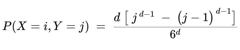
[ \huge \frac{d}{6} ;\times;\left(\frac{1}{6}\right)^{d-1};\bigl[j^{d-1} - (j-1)^{d-1}\bigr] ;=; \frac{d,\bigl[j^{d-1} - (j-1)^{d-1}\bigr]}{6^{d}}. ]
Hence the simplified form is
[
\huge P(X = i, Y = j) ;=; \frac{d,\bigl[j^{d-1} - (j-1)^{d-1}\bigr]}{6^{d}} \quad\text{for }i>j. ]
Edge Cases and Consistency Checks
Range of i, j: We must have 1 <= j <= i <= 6. The formula for (P(X=i,Y=j)) is valid only for (i>j). The separate formula for (X=i, Y=i) covers the case (i=j).
Summation to 1: If you sum (P(X=i, Y=j)) over all (1 \le j \le i \le 6), it should equal 1. One can verify this by partitioning the sample space based on the maximum and second-highest values.
Boundary cases:
If (i=1), then automatically (X=1) and (Y=1) with probability ((1/6)^d). Indeed, plugging (i=1) into the formula for (P(X=1, Y=1)) yields (\frac{1^d - 0^d - d(0)^{d-1}}{6^d} = \frac{1}{6^d}).
If (i=6) and (j=5), then you can check that (\frac{d[5^{d-1} - 4^{d-1}]}{6^d}) captures the scenario exactly one die is 6, at least one is 5, etc.
Interpretation of Y = X: Whenever we have 2 or more dice at the top value (i), we get (Y=i). The formula for (P(X=i, Y=i)) explicitly accounts for at least two dice taking the maximum value.
Possible Interview Follow-up Questions
1) How would you simulate this distribution in code to empirically verify it?
You could run a large Monte Carlo simulation, counting the frequency of outcomes ((X,Y)) and compare with the theoretical probabilities.
An example in Python:
import random
from collections import Counter

def simulate_joint_distribution(d, trials=10_000_00):
    """
    d is the number of dice
    trials is how many times we roll all d dice
    returns empirical frequency of (X, Y)
    """
    counts = Counter()
    for _ in range(trials):
        roll = [random.randint(1, 6) for _ in range(d)]
        max_val = max(roll)
        # Count how many times max_val appears
        count_max = roll.count(max_val)
        if count_max >= 2:
            # second-highest is also the same as max_val
            second_highest = max_val
        else:
            # one die is max_val, so we look for the max among the rest
            second_highest = max(val for val in roll if val != max_val)
        counts[(max_val, second_highest)] += 1

    # Convert counts to probabilities
    return {k: v / trials for k, v in counts.items()}

# Example usage
d = 3
empirical = simulate_joint_distribution(d)
# Now empirical[(i, j)] should be close to the theoretical probability
Then you could compare empirical[(i, j)] with the closed-form expressions:
For i=j, compare with
(i^d - (i-1)^d - d*(i-1)^(d-1)) / 6^d.For i>j, compare with
d * [ j^(d-1) - (j-1)^(d-1) ] / 6^d.
2) Why does exactly one die being the maximum exclude the possibility Y = X?
If exactly one die attains the maximum (i), then no other die can be (i). By definition, the second-highest value must be strictly less than (i). Hence that scenario belongs to (X=i, Y < i).
3) Is it possible for Y > X in any circumstance?
No, by definition we label (X) as the highest. So (Y) cannot exceed (X).
4) How do these formulas change if the dice are not fair?
If each face has a (possibly different) probability (p_k) for face value (k) (where (k) in {1,...,6}), the combinatorial reasoning is similar but the expressions become more complicated. Instead of factors like (1/6) for each die, you would have the probability of face (i) for the highest or second-highest dice, and sums over ways the remaining dice distribute themselves among the smaller faces. The logic is the same, but each outcome has a product of probabilities depending on how many dice show each face.
5) Could you use an alternative approach using order statistics for discrete distributions?
Yes. (X) and (Y) can be viewed as the top two order statistics in a sample of size (d). Order statistics for discrete distributions can be computed systematically by enumerating possible outcomes. The binomial-based expansions we used are essentially one direct combinatorial approach to the distribution of the maximum and second-maximum. For continuous distributions, we typically rely on the PDF of the order statistic. For discrete dice, direct combinatorial sums are simpler.
6) In an ML or data science context, can you think of a scenario where you might need such a distribution?
One example is in analyzing “top-K” metrics, where we look at the top scoring predictions from a multi-output model. Another context is game simulation, where many dice are rolled and you track the top or near-top results. Sometimes in Bayesian modeling with discrete priors, we might care about the highest and second-highest posterior samples.
All these use cases revolve around “order statistics” in discrete contexts, quite relevant in certain simulation-based or generative models.
Below are additional follow-up questions
Another Potential Follow-Up Question: How can we extend this result to the top three (or top K) highest values?
In some applications, you might need the joint distribution of the top three scores or, more generally, the top K scores out of d dice. The logic here can be extended, but it becomes more intricate because you have additional conditions about exactly how many dice attain each of the top values.
To find (P(X_1 = a, X_2 = b, X_3 = c)) for distinct values (a > b > c), you need to count the number of dice hitting (a), (b), (c), and also ensure all other dice are below (c). Additionally, you handle the cases where some of these top values coincide if you allow ties (e.g., the third-highest might equal the second-highest if multiple dice show that second-highest score). Each outcome is a combinatorial partition of the d dice with carefully enumerated probabilities for each face outcome. The main pitfall is that the combinatorial expressions grow more complicated. In real-world usage, it’s easy to mix up when ties occur or to accidentally double-count scenarios, so double-check each tie condition (like “top two are tied, but the third is strictly smaller,” etc.). A robust approach involves systematically enumerating how many dice show each of the top values and making sure the rest are strictly smaller, but the complexity can become large for bigger K.
In practice, a common subtlety is undercounting or overcounting configurations with multiple ties. One potential real-world issue occurs if you have to implement these formulas in code for large d and want to sum all possible combinations for top K: you need to keep track of potential integer overflow if you use naive multiplicative counting. To avoid such pitfalls, people often rely on dynamic programming or well-chosen generating functions.
Another Potential Follow-Up Question: How would you derive the distribution of the difference X - Y?
Sometimes one might want to know how far apart the highest and second-highest scores are on average. You can define a new random variable (D = X - Y) and compute its distribution by summing (P(X=i, Y=j)) over all i, j such that (i - j = d). In other words, (P(D = d)) is the sum of (P(X = i, Y = j)) over all i, j with i - j = d.
Specifically,
(D = 0) corresponds to the event that at least two dice tie for the highest value. So (P(D=0)) is (\sum_{i=1}^{6} P(X=i, Y=i)).
(D = k) for k > 0 means exactly one die is i and at least one is j where i = j + k.
A major pitfall is forgetting that if X = Y, you only contribute to D=0, and if X > Y, you contribute to a strictly positive difference. Another subtlety is ensuring the domain of D is from 0 up to 5 (since the maximum difference between two faces on a six-sided die is 5). In real scenarios, one might be tempted to ignore the possibility of ties and just compute the distribution of the gap from a continuous viewpoint, which would be incorrect for a discrete die. This leads to underestimating the probability of zero gap if you forget about the tie scenario.
Another Potential Follow-Up Question: How can we compute P(X = i) directly, and does it match with summing over j in P(X = i, Y = j)?
One interesting check is computing (P(X = i)) in two ways:
Using the standard result that the probability the maximum is exactly i is [ \huge P(X = i) = \left(\frac{i}{6}\right)^d - \left(\frac{i-1}{6}\right)^d. ]
Summing (P(X = i, Y = j)) over j = 1 to i.
These must coincide because (X = i) is the union of events ({Y=1}, {Y=2}, \dots, {Y=i}). The sum
[ \huge \sum_{j=1}^{i} P(X=i, Y=j) ] should match the simpler expression for (P(X=i)). This is a helpful internal consistency check. A subtlety is carefully including the case j = i, which you must not omit. In a real interview, you might be asked to show that this summation indeed resolves to the known closed-form for P(X = i). Failing to include the tie scenario (j = i) is a common mistake that leads to partial sums and confusion.
Another Potential Follow-Up Question: Does the distribution of (X, Y) change if we perform sequential rolls rather than rolling all dice simultaneously?
Mathematically, it does not. Rolling d dice at once or rolling them one at a time (assuming each roll is an independent fair six-sided die) yields the same joint distribution for (X, Y). Independence of the dice rolls and identical distribution ensures the outcome is the same regardless of how you schedule the rolls. A subtle real-world scenario might arise if the rolling is done in a dependent way—for instance, if we had a rule that once a certain value is rolled, subsequent rolls cannot exceed it. That would alter the distribution. In standard settings of fair and independent dice, the distribution is the same. The main pitfall is incorrectly injecting a time dependence on the assumption that rolling in a sequence changes the overall distribution.
Another Potential Follow-Up Question: How to handle the situation when d = 2?
When d = 2, the second-highest value Y will always be equal to X because there are only two dice. So the event “exactly one die has the maximum and the other is strictly smaller” does not occur in the sense of forcing Y < X. Actually, for d = 2, we either have both dice the same (in which case X = Y), or one die is larger (then that is X) and the other is smaller (that is Y). But crucially, the definition says Y = X if and only if two or more dice yield the highest score. Here, with only two dice, if they differ, the second-highest is strictly less. If they are the same, then X = Y.
The subtlety is remembering that the same formula still works:
For i = j, (P(X = i, Y = i)) with d=2 means both dice are i, which is ((1/6)^2).
For i > j, it means one die is i, the other is j. The probability is 2 * (1/6)*(1/6) = 2/36 if i != j. Summing appropriately over i>j recovers the total of 1 minus the sum of probabilities that the two dice are equal. A real-world pitfall is mixing up the condition Y = X “only if at least two dice show the top value.” With exactly 2 dice, that means Y = X precisely when both dice match.
Another Potential Follow-Up Question: Are X and Y ever approximately independent for large d?
For large d, there might be an intuition that “once the maximum is large, the second-highest might be fairly large as well,” but X and Y remain correlated (they are definitely not independent) because if X is extremely high, it is more likely Y is also high. For instance, if you know X = 6 and there are many dice, it is more probable that at least one more die also hit a 6, making Y = 6 more likely. So in the limit as d goes large, the distribution of X and Y skews toward 6, but in a correlated fashion: we are more likely to get multiple 6s. A naive pitfall is to assume that with more dice, the random variables might “decorrelate,” but that is not the case here because knowing the maximum is 6 significantly influences the probability that the second-highest is also 6.
In a real-world analytics setting, making an independence assumption about order statistics can lead to erroneous predictions or intervals. The takeaway is that order statistics for discrete distributions typically remain correlated because the events “the maximum is i” and “the second maximum is j” are interdependent.
Another Potential Follow-Up Question: How does the result change if the faces are from 1 to M instead of 1 to 6?
Many dice-based scenarios generalize to an M-sided die. The combinatorial framework is the same, but each (1/6) factor changes to (1/M). For instance:
(P(X = i, Y = i)) would be [ \huge \sum_{r=2}^{d} \binom{d}{r}\left(\frac{1}{M}\right)^r \left(\frac{i - 1}{M}\right)^{d-r} ] which can again be simplified using expansions analogous to the 6-sided case but with M in place of 6.
(P(X = i, Y = j)) for i > j becomes [ \huge \frac{d \Bigl[j^{,d-1} - (j-1)^{,d-1}\Bigr]}{M^d} ] just replacing 6 by M.
A subtlety is that i, j now range from 1 to M. If you do any expansions or sums, be sure you adapt your upper bounds. In real-world usage, confusion sometimes arises if M is large, e.g., in computing distributions for discrete variables with more than 6 outcomes. As M grows, numeric overflow or complexity might become more significant. Additionally, if M is not prime or if the distribution of faces is not uniform, you’d have to adapt these formulas to the more general case.
Another Potential Follow-Up Question: Could partial knowledge about the dice outcomes affect the distribution of X, Y?
Yes. Suppose you learn that 3 out of 5 dice show a 6, but the remaining two are unknown. Then the distribution of (X, Y) changes conditionally, because you already know that there are multiple 6s. You automatically know X = 6 and Y = 6, and there’s no uncertainty left about X and Y in that scenario. Or, if you learn some dice cannot exceed 3 due to a constraint, you must recompute the distribution given that partial constraint.
A common pitfall is ignoring the conditioning and still using unconditional probabilities. In real-world gaming or data situations, you might be combining partial observations with prior knowledge, in which case the unconditional formulas for (P(X = i, Y = j)) no longer apply directly. Instead, you must compute conditional probabilities given the observed partial outcomes. This can be handled with Bayes’ Theorem or direct enumeration of the remaining unknown dice, but incorrectly mixing unconditional and conditional probabilities is a typical mistake that leads to inconsistent results.