ML Interview Q Series: K-Means Centroid Updates Using Batch and Stochastic Gradient Descent.

📚 Browse the full ML Interview series here.

What is the loss function used in k-means clustering for k clusters and n sample points? Compute the update formula using 1) batch gradient descent, 2) stochastic gradient descent for the cluster mean for cluster k using a learning rate ε.

Loss Function in k-means Clustering

The k-means algorithm partitions a dataset of nn points {x1,x2,…,xn} into k clusters. Each point xi​ is associated with exactly one cluster. Denote the cluster means (centroids) by {μ1,μ2,…,μk}. The standard objective (loss) function is the sum of squared Euclidean distances of each point to its assigned cluster’s mean:

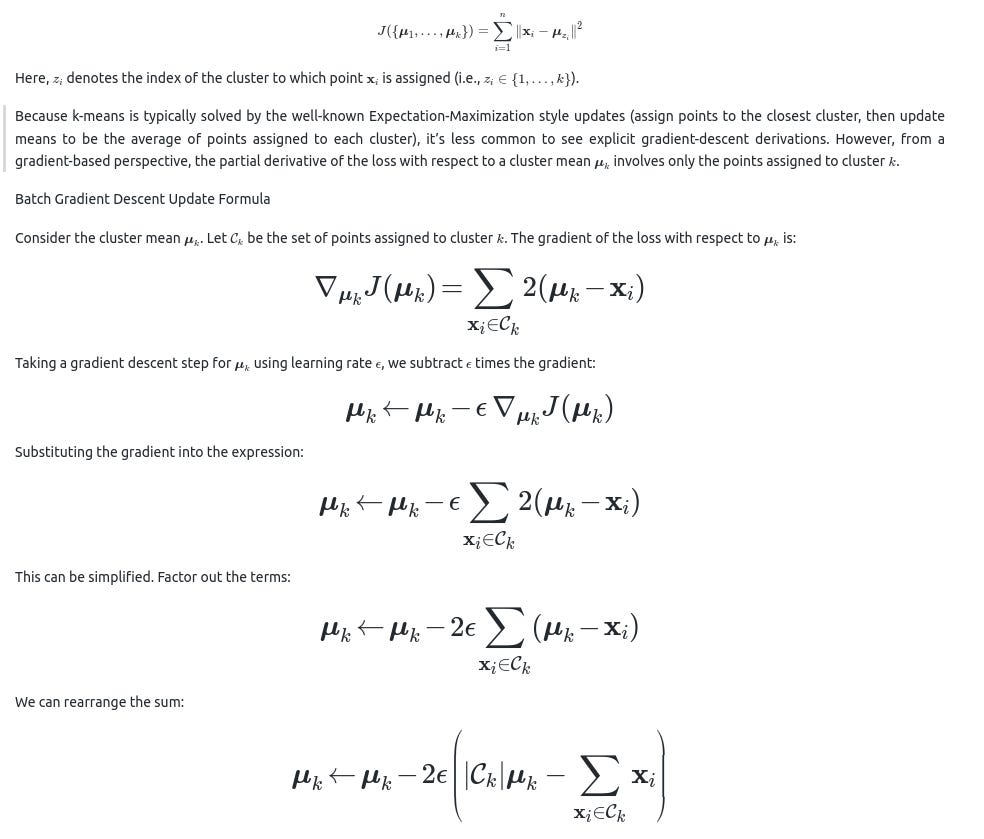
The intuition is that for each sample, we make a small move of μk​ toward xi​. If we choose very small learning rates and repeatedly sample points within each cluster assignment, over time the mean drifts to the actual average. But typical k-means does not usually adopt SGD for centroid updates because it’s more direct to average all points in a cluster. However, for streaming or very large-scale scenarios, SGD-like updates can be useful.

Example Python Code for a Single SGD Step

Below is a minimal illustration of how you might implement a single stochastic gradient step for a cluster mean μkμk​, given one data point xx that belongs to cluster kk. The variable mu_k represents μkμk​, x represents the chosen point xx, and epsilon is the learning rate:

import numpy as np

def sgd_update(mu_k, x, epsilon):
    gradient = 2 * (mu_k - x)
    mu_k = mu_k - epsilon * gradient
    return mu_k

# Example usage
mu_k = np.array([1.0, 2.0])
x = np.array([2.0, 3.0])
epsilon = 0.01

new_mu_k = sgd_update(mu_k, x, epsilon)
print("Old mu_k:", mu_k)
print("New mu_k:", new_mu_k)

Potential Follow-up Questions and Detailed Answers

How do we initialize the means in k-means to reduce the risk of poor local minima?

Initialization can significantly impact the final clustering. A common naive strategy is to randomly pick (k) points from the dataset as the initial centroids. However, this can lead to suboptimal solutions if the chosen points are close together or unrepresentative of the overall distribution. A well-known improvement is the k-means++ algorithm, which selects initial centroids in a way that spreads them out in feature space. Specifically, it picks the first centroid uniformly at random from the data, then chooses subsequent centroids with probability proportional to the squared distance from the already chosen centroids. This approach significantly reduces the probability of ending in a bad local optimum and often converges faster.

In more advanced or streaming scenarios, alternative initialization methods such as random partition or hierarchical clustering-based initializations can be employed. In practice, multiple runs with different initial conditions can also help identify a better minimum.

What if a cluster ends up with no points assigned during the iteration?

It can happen, especially if one cluster center is placed in a region that is not “closest” to any data point. The standard approach is to either (1) re-initialize that cluster center to a random data point or (2) pick the point that is farthest from its current centroid among the largest cluster. The second method tries to break up large clusters to ensure each cluster remains active. Ensuring every cluster has at least one point is essential, because the mean of an empty cluster is undefined, and that cluster will never move unless it is re-initialized or assigned points in some way.

How do you handle very large datasets for k-means?

Computational complexity can be high for large (n). Standard k-means requires repeated passes over the dataset, and each iteration can be expensive. A few popular solutions:

Use mini-batch k-means. Instead of using all data points in each iteration, sample a mini-batch. Each step updates the means with these few samples. It’s a stochastic gradient approach, but in practice it converges quickly.

Use an approximate nearest neighbor search or a pre-clustering approach. Methods like k-means|| (k-means parallel) or hierarchical clustering can reduce the dataset size or help with better initialization.

Use advanced data structures for distance computations or approximate algorithms (like the kd-tree for certain dimensionalities, though not always beneficial in high dimensions).

How does the choice of distance metric affect the algorithm?

Classic k-means uses Euclidean distance. The loss function is the sum of squared Euclidean distances. If you use a different distance metric (for instance, Manhattan distance), the centroid update formula changes. For Manhattan distance, the best “centroid” is actually the median of the assigned points, not their mean. More generally, with the ℓ2​ norm, the mean is the minimizer of squared errors. For the ℓ1​ norm, the median is the minimizer of absolute errors. If a specialized distance measure is introduced, the notion of a centroid could change significantly, and you might need custom update rules or a different algorithm entirely (such as k-medoids).

Can k-means handle non-spherical clusters or clusters of very different sizes?

k-means inherently prefers clusters that are roughly spherical (equal variance in all directions). If the data distribution has elongated clusters, or clusters with varying densities, k-means may not yield good results. In such cases, alternative clustering methods such as DBSCAN, spectral clustering, Gaussian mixture models, or density-based methods might handle such shapes and scales better.

If domain knowledge suggests that clusters are spherical, k-means is a strong candidate due to its conceptual simplicity and speed. Otherwise, you may need to incorporate additional steps (for instance, standardizing or normalizing each feature, using other distance metrics, or switching to a more robust algorithm).

Why do we often avoid explicit gradient descent for k-means and instead use the iterative assignment-and-update procedure?

The direct iterative approach used by classic k-means alternates between:

• Assigning each point to the nearest cluster center.

• Recomputing cluster centers by taking the mean of the points in each cluster.

This approach is effectively coordinate descent on the same objective and typically converges faster for this specific discrete–continuous minimization problem. In fact, the cluster assignments and the means have closed-form update rules if we keep one fixed while updating the other. Using general gradient descent is more general but often converges more slowly for the special structure of k-means.

How do we address local minima in k-means?

The k-means objective function is non-convex in the joint space of cluster assignments and means. It’s convex in the means if assignments are fixed, and vice versa, but not jointly. Consequently, local minima are common. Strategies to mitigate local minima include:

Multiple random initializations, then pick the best clustering result.

Smarter initialization like k-means++ to reduce the chances of a poor local minimum.

Running variations of k-means with modifications (like simulated annealing or random swaps) can help escape some local minima.

Could we use momentum or more advanced optimizers for the gradient-based approach?

In principle, yes. Instead of performing plain gradient descent updates to μk​, one could use momentum-based gradient descent (e.g., use a moving average of gradients) or optimizers such as Adam. In practice, the standard k-means iterative procedure is typically more efficient. But for extremely large, streaming data or specialized scenarios, momentum or adaptive step-size methods might help refine the centroids as new data arrives.

How do we handle outliers?

k-means is sensitive to outliers because the mean is heavily affected by extreme values. If the dataset contains outliers, they may pull the centroid away from the main bulk of points, degrading cluster quality. Common mitigation strategies:

Preprocessing or removing outliers if domain knowledge allows.

Using a robust distance measure or a robust version of k-means (e.g., k-medoids or trimmed k-means, which ignores a certain percentage of extreme points).

Applying transformations (e.g., log transform) to mitigate extreme values.

How do we implement an online or streaming version of k-means?

An online approach processes data in small batches or even one point at a time:

Initialize cluster means (e.g., randomly pick from the first few points, or use k-means++ on a small initial sample).

For each incoming point (or mini-batch):

• Determine which cluster is closest.

• Update the corresponding centroid using a small step (SGD update) toward the point.

This helps maintain running estimates of cluster means and can handle potentially unbounded data streams without storing the entire dataset in memory. The learning rate might be decayed over time so that earlier cluster assignments have more influence, or it might be kept constant if the distribution is changing, depending on the application.

How do we interpret partial derivatives in k-means, given that cluster assignments are discrete?

Technically, the full k-means objective with discrete assignments is not purely differentiable with respect to μk​ and the cluster memberships simultaneously. The standard analysis of partial derivatives is done by assuming the assignments are temporarily fixed. Once assignments are decided (e.g., by “hard” nearest-centroid classification), the portion of the objective that matters for μk​ is simply the sum of squared distances to the points in cluster k. That is differentiable with respect to μk​. Then, the algorithm updates μk​ to the gradient-based optimum.

The non-differentiability arises from the cluster membership function (which is effectively a step function in continuous space). But k-means splits the optimization problem into two steps, each of which is simpler and (locally) converges to a stationary point.

Could the gradient-based view help with soft assignments?

Yes. If you generalize k-means to a Gaussian mixture model and use maximum likelihood estimation, you end up with a soft assignment of points to clusters (each point has a probability of belonging to each cluster). That problem can be solved with the Expectation-Maximization (EM) algorithm for Gaussian mixtures. The means update step becomes:

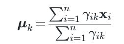
where γik​ is the soft assignment (posterior probability) of point ii belonging to cluster k. This is differentiable in a more standard sense, and we can interpret the EM steps as coordinate ascent in the expected complete data log-likelihood. One could indeed use gradient-based methods for mixtures, but the EM algorithm is typically the method of choice.

How does the dimensionality of the data affect k-means?

As dimensionality grows, distance metrics can become less discriminative (the “curse of dimensionality”). Points may appear nearly equidistant from each other, causing poor cluster separation. k-means still tries to minimize squared distances, but often performance deteriorates in very high dimensions. Common remedies:

Dimensionality reduction (PCA, autoencoders, etc.) to project data into a lower-dimensional space.

Feature selection to retain only the most salient dimensions.

Using domain knowledge or specialized metrics if certain dimensions are known to be noisy or irrelevant.

Below are additional follow-up questions

What if some features have very different scales or units in k-means, and how do we address that?

One subtle but significant pitfall arises when different features are measured in different scales or units (for instance, one feature might be in kilometers, another in grams, another in a ratio). k-means uses the Euclidean distance, so features that have larger numeric ranges or units can dominate the distance computation and overshadow features with smaller numeric ranges. This can distort cluster assignments because points may appear “further apart” primarily along large-scale features.

Approach to Addressing Different Scales

• Normalization/Standardization: Commonly, we standardize each feature to have zero mean and unit variance, or we rescale them to a specific range (e.g., [0, 1]). This ensures that each dimension contributes more equally to the distance measure.

  Domain-Dependent Transformations: If some features have outliers or long-tail distributions, applying a log transform (for positive features) or other nonlinear scalings can sometimes help.

• Potential Pitfalls: Over-normalizing can destroy some domain-specific interpretability. If a certain feature is truly more critical for the clustering objective, forcibly scaling it down might lose meaningful distinctions. So, standardization is typically beneficial, but it should be balanced with domain knowledge.

Edge Cases

• If a feature is constant for all data points, it provides no separation and might be dropped.

• Extremely high-dimensional data with varying scales can lead to difficulty choosing the right normalization scheme, especially if feature ranges differ by orders of magnitude.

Example If we have a dataset with features [height in cm, weight in kg, shoe size in US measure], we might first standardize each dimension across all samples:

where μj​ and σj​ are the mean and standard deviation of feature j. This step can drastically improve k-means performance by preventing any single feature from dominating the distance.

---

How do we evaluate or measure the performance or quality of clusters after running k-means?

While k-means has an internal objective (the sum of squared distances within clusters), there are times we want external or other internal metrics to assess cluster coherence and separation. The within-cluster sum of squares (inertia) decreases with more clusters, so we often need additional measures.

Common Cluster Quality Metrics

• Silhouette Coefficient: Measures how similar a point is to points within its own cluster vs. points in other clusters. The silhouette coefficient for each sample is

  

  where (a_i) is the average intra-cluster distance for point (i), and (b_i) is the minimum average distance to other clusters. A higher silhouette (close to 1) indicates well-separated and cohesive clusters.

• Davies-Bouldin Index: Considers within-cluster scatter vs. between-cluster separation. Lower is better.

• Calinski-Harabasz Index: Ratio of between-cluster dispersion to within-cluster dispersion. Higher is better.

• External Metrics: If you have ground-truth labels, you can compute metrics like adjusted Rand index, normalized mutual information, or clustering accuracy.

Potential Pitfalls

• Relying solely on the k-means objective might push for more clusters than necessary (adding more clusters will almost always reduce the sum of within-cluster squares).

• Some metrics like silhouette might be misleading in certain data distributions. For instance, data with overlapping clusters or complex shapes can show suboptimal values.

• Real-world data may not have ground-truth labels, so external measures can’t be computed, leaving only internal measures which can still be ambiguous.

  Edge Cases

  • Extremely large or high-dimensional data can cause certain metrics (like silhouette) to behave poorly or require significant computation.

  • Clusters with very few points can skew the metrics, especially silhouette, which might produce inflated or degenerate values.

  ---

  How can we speed up the assignment step in k-means when the dataset is large, without significantly sacrificing accuracy?

  The assignment step in k-means requires, for each point, computing the distance to each centroid. This is O(n×k)O(n×k) per iteration. For large nn and moderately large kk, this step dominates the computational cost.

  Methods to Speed Up

  Approximate Nearest Neighbor (ANN): Use spatial data structures or libraries (e.g., annoy, FLANN) for approximate nearest centroid search.

• Mini-Batch k-means: Only process small batches of data points at each iteration, which dramatically cuts down the distance computations.

• Using Clustering Trees or KD-trees: In lower dimensions, tree-based methods can prune distance checks. However, in high dimensions, kd-trees degrade in performance.

• Hierarchical Approaches: Partition the data into small “pre-clusters” and only do expensive distance checks for local neighborhoods.

Potential Pitfalls

• Approximate methods may sometimes assign points to the wrong centroid if the approximation is poor. This can degrade solution quality or converge differently.

• Data structures like kd-trees become less effective as dimensionality grows.

• If the mini-batch is not representative, updates might be biased, requiring more iterations.

Edge Cases

• Very high-dimensional data might require specialized approximate methods; straightforward indexing might fail.

• If memory is extremely limited, storing large structures for approximate search might also be infeasible, requiring streaming or chunked approaches.

---

How do we handle constraints such as “these points must be in the same cluster” or “these points must be in different clusters” in k-means?

Sometimes we have partial or domain-specific constraints that certain points belong together (must-link) or must not belong together (cannot-link). Plain k-means does not account for such constraints.

Constrained k-means / Semi-Supervised Clustering

• Must-link Constraints: The algorithm enforces these points to go to a single centroid, effectively merging them in the assignment step. Sometimes a subroutine ensures that after assigning each point to its closest centroid, any must-link pairs that ended up in different clusters trigger reassignments.

• Cannot-link Constraints: This ensures certain pairs cannot share the same centroid. After the standard assignment step, if any pair violates the constraint, a forced reassign or centroid adjustment is triggered.

Algorithmic Adjustments

• Penalty-based Approach: One can modify the objective function to add a penalty term for violating constraints, then solve with a suitable iterative approach.

• Search/Heuristic: Constraint checks are included after normal assignment to fix any violations, though this can lead to slower convergence.

Potential Pitfalls

• Hard constraints can lead to conflicting assignments if the data distribution strongly suggests different cluster structures.

• Overly strict constraints can force very unnatural centroids and degrade the overall clustering performance.

• Implementation complexity is higher, especially if there are many constraints.

Edge Cases

• If must-link constraints form large chains, effectively all points in that chain must be in one single cluster, which can overshadow data-driven assignments.

• Conflicting constraints (e.g., a must-link chain that contradicts a cannot-link pair) make it impossible to satisfy all constraints. This necessitates relaxing constraints or weighting them.

---

How do we label or interpret the resulting clusters once k-means has converged?

K-means outputs cluster assignments and centroids but does not provide direct semantic labels (e.g., “cluster 1 is dogs, cluster 2 is cats”). Interpreting these clusters is crucial, especially in business or research contexts.

Methods for Labeling or Interpreting Clusters

• Inspect Centroids: Examining centroid coordinates can provide insight, especially if certain features dominate. In higher dimensions, consider dimensionality reduction or cluster prototypes.

• Look at Representative Points: For each cluster, identify the points closest to the centroid (cluster exemplars). These exemplars can highlight the main characteristics of that cluster.

• Analyze Feature Importances: If available, compute which features have the greatest variance within or across clusters. This might guide a human analyst to name or interpret clusters.

• Domain Knowledge: Map the cluster centroids or exemplars back to domain-specific categories.

Potential Pitfalls

• High-dimensional clusters might be difficult to interpret because the centroid does not reflect a “real” data point, but rather an average.

• If the dataset is heavily imbalanced, some clusters might be extremely small or large, and interpretation might be skewed by the large cluster.

Edge Cases

• Clusters with only a handful of points might be outliers rather than meaningful “topics” or classes.

• In purely numeric data with no domain knowledge, labeling might be arbitrary. One must rely on patterns in the feature space or additional metadata.

---

How do we adapt k-means if the data distribution changes over time (concept drift) in a streaming environment?

In many real-world applications (e.g., event data, sensor data, user behavior logs), the underlying distribution can drift over time. A fixed set of centroids learned on historical data may no longer be relevant.

Online or Streaming K-means

• Incremental Updates: Continuously update centroids with each new data point or small mini-batches. For a new point xi​, find the nearest centroid μk​ and do an SGD-like update:

  

  Decaying Learning Rate: Gradually decrease ϵϵ so older data points matter less if the distribution is stable. If concept drift is ongoing, keep ϵ at a small positive value so the algorithm can adapt.

• Windowing: Maintain a moving window of recent data. Cluster only that subset, discarding older data or weighting it less.

Potential Pitfalls

• Too large a learning rate can cause the centroids to swing wildly with new data, causing instability.

• Too small a learning rate might make the algorithm unresponsive to actual shifts in distribution.

• If the drift is sudden (abrupt distribution change), incremental updates might be too slow, requiring re-initialization.

Edge Cases

• Seasonality or cyclical patterns might confuse a purely incremental approach. One might need advanced drift detection methods to decide when to reset or shift centroids more aggressively.

• If new clusters appear in the data stream, a fixed (k) might not suffice, requiring dynamic addition or removal of centroids.

---

How do we choose the optimal number of clusters (k) in k-means beyond elbow or silhouette methods?

While common heuristics exist—like the elbow method (plotting the within-cluster sum of squares vs. (k)), silhouette analysis, or domain-based guesses—sometimes these are inconclusive or lead to ambiguous decisions.

Advanced or Alternative Methods

• Gap Statistic: Compares the within-cluster dispersion to that expected under a reference distribution (often uniform or a bootstrapped sample). The chosen (k) maximizes the gap between the actual data’s dispersion and that of the reference.

• Information Criteria: For Gaussian mixture models, methods such as Bayesian Information Criterion (BIC) or Akaike Information Criterion (AIC) can guide selecting the number of components. Though not strictly k-means, they can be adapted in some ways.

• Stability Analysis: Repeatedly cluster subsamples of the data. The best (k) is the one that yields the most stable partitions across these subsamples.

Potential Pitfalls

• The elbow method might not always show a clear or sharp bend, leading to subjective choices.

• Some advanced methods can be computationally expensive because they involve multiple re-clusterings or references.

• Domain knowledge might override purely statistical measures—sometimes a domain requires a certain number of meaningful groupings.

Edge Cases

• Very large (k) might lead to over-partitioning (clusters with only a few points).

  Very small (k) might oversimplify the data. For instance, if the domain obviously has 20 categories but a heuristic suggests (k=2), the results could be unhelpful.

---

How do we handle categorical or mixed-type data (both numeric and categorical) in k-means?

k-means relies on the Euclidean distance, which is not strictly meaningful for categorical variables (e.g., color = “red,” “blue,” “green”). Mixed-type data complicates direct distance calculations.

Variations and Alternatives

• k-modes: Replaces the mean-based centroid with a mode-based centroid for categorical features, and uses a matching-based distance measure.

• k-prototypes: Combines numeric and categorical data by mixing k-means and k-modes concepts. Numeric features are updated by means, while categorical features are updated by modes.

• Feature Encoding: One-hot encoding or embeddings for categorical variables to approximate them as numeric. Then, apply standard k-means. But this can inflate dimensionality or distort distances.

  Potential Pitfalls

  • One-hot encoding can cause the distance metric to be dominated by the large number of binary features.

  • Overly simplistic distance metrics on categorical variables (like 0 if matching, 1 if not) might fail to capture partial similarities.

  • If numeric features vary widely in scale while categorical variables are used with a simplistic distance, the numeric portion might overshadow the categorical portion.

  Edge Cases

  • Rare categories might pose a challenge. If a category is present in just a few data points, the algorithm might isolate those points or incorrectly merge them into a large cluster.

  • Mixed-type data that includes, for example, textual descriptions, ordinal features, and continuous features requires a carefully designed distance measure or specialized clustering method.

    How do we detect if k-means is stuck in a degenerate solution where multiple centroids converge to the same point?

    A degenerate situation occurs when two or more centroids end up at identical coordinates. This usually indicates that the algorithm assigned the same set of points (or near the same set) to multiple clusters. It can lead to fewer effectively distinct clusters than (k).

    Indicators of Degeneracy

    • Checking after each iteration if any centroids coincide. If so, the algorithm might not progress in a meaningful way with those duplicated centroids.

    • Tracking cluster sizes: if certain clusters have zero points assigned, that centroid might eventually move to an identical location as another centroid.

    Mitigation Strategies

    • Re-initialize the Duplicate Centroid: If a centroid collapses into another, reassign it to a different, unoccupied region or randomly pick an unassigned point as the new centroid.

    • Examine the Data: If the data distribution has extremely dense subregions, multiple centroids might converge there. This could be a sign that (k) is too high or the initialization was unlucky.

    Potential Pitfalls

    • Automatic re-initialization can cause the algorithm to jump around unpredictably, potentially increasing iteration time.

    • In high-dimensional or sparse data, multiple points might effectively be “tied” in distance, leading to unusual centroid placements.

    Edge Cases

    • If the dataset truly has fewer distinct clusters than (k), duplicates might be unavoidable. The final solution might effectively have fewer unique clusters.

    • Some advanced methods (like k-means++) mitigate, but do not entirely eliminate, the possibility of degeneracy.

    ---

    How does k-means handle severely imbalanced clusters or data with a massive cluster and tiny clusters?

    In real-world scenarios, data distributions are often skewed: one cluster might contain the majority of points, while other clusters are very small. Classic k-means tries to minimize the overall sum of squared distances, which can favor fitting the large cluster well and might place less emphasis on smaller clusters.

    Consequences for Imbalanced Data

    • Small clusters might get merged into a single centroid or be pulled toward the large cluster if they are not sufficiently distinct.

    • A cluster with very few points might not significantly affect the overall objective, so the algorithm can underfit it.

    Possible Remedies

    • Weighted k-means: Assign higher weight to points in underrepresented clusters to make them contribute more to the objective.

    • Oversampling or Data Augmentation: If appropriate, replicate or synthesize minority cluster points so the algorithm treats them more equitably.

    • Ensemble Clustering: Combine multiple runs or different sampling strategies to ensure minority structures are captured.

    Potential Pitfalls

    • Oversampling artificially can distort the distribution if you don’t do it carefully.

    • Weighted k-means requires specifying weights, which might be unknown or guessed.

    • A large cluster might truly dominate the distribution, and forcing more balanced clusters could be counterproductive.

    Edge Cases

    • If an extremely small cluster is just an outlier group, the algorithm might create a single centroid for outliers. Whether that is desired depends on your application (sometimes outliers should be identified separately).

    • If the large cluster is extremely heterogeneous internally, it might be more naturally broken into multiple clusters, even though that might not be the global optimum for a small (k).

    ---

    How do we debug or diagnose k-means results that do not match domain expectations?

    It is not uncommon for the final clustering to disagree with a domain expert’s expectation (e.g., “I expected all these items to group together, but the algorithm put them in separate clusters”).

    Debugging Steps

    • Check Data Preprocessing: Ensure that data was normalized or standardized if needed, that missing values were handled properly, and that no features dominate incorrectly.

    • Check Initialization: If the initial centroids are poorly chosen, results can diverge from domain intuition. Try k-means++ or multiple restarts.

    • Examine Each Cluster in Detail: Inspect the points in each cluster, look for patterns that might explain the unexpected grouping (perhaps a subtle feature dominated the distance metric).

    • Perform Dimensionality Reduction: Visualize clusters in 2D or 3D using something like PCA or t-SNE to see if the separation is actually coherent in the reduced space.

    Potential Pitfalls

    • Domain knowledge might rely on different measures of similarity than Euclidean distance. If experts think “these items belong together,” but that notion of similarity is not captured by the numeric features, k-means might produce “unexpected” results.

    • Overlooking data corruption or mislabeled features can lead to bizarre clustering.

    Edge Cases

    • If domain knowledge strongly disagrees with k-means, it might be that the data is missing crucial features that define the desired grouping.

    • k-means might have found a local minimum that is valid for the data representation but does not align with the domain’s conceptual categories (a mismatch between the domain’s concept of cluster structure and the purely geometric notion used by k-means).

    ---

    How do we incorporate prior knowledge or partial supervision into the centroid update without strict must-link or cannot-link constraints?

    Sometimes, we have “soft” prior knowledge: for example, we suspect cluster centers to lie near certain regions, or we want to nudge them in a particular direction without completely enforcing constraints.

    Possible Approaches

    • Regularization Term: Add a term to the objective that penalizes deviations from known or hypothesized centroid locations. For instance, if we want centroid μk​ to stay near a reference point νk​, add

      

      to the loss, with λ controlling the strength of the prior.

    • Initialization Bias: Initialize centroids near regions suggested by domain experts, but let standard k-means proceed. This can lead to solutions that remain in the vicinity of those initial guesses.

    • Weighted Data Points: If certain points are believed to be prototypes, assign them a higher weight so they pull the centroid more strongly in that direction.
      

    Potential Pitfalls

    • Overly large λ in a regularization approach can override the actual data distribution.

    • Biased initialization can cause the algorithm to converge to suboptimal solutions if the domain experts’ guess was incomplete or partially incorrect.

    Edge Cases

    • If the “prior” clusters conflict with the structure in data, the algorithm might produce solutions that satisfy neither perfectly.

    • Weighted data points might cause significant distortion if the domain knowledge is inaccurate or if weighting is done too aggressively.

    ---

    How do we determine if k-means is the right clustering method compared to density-based or model-based clustering approaches?

    While k-means is popular and computationally efficient, it might not always be suitable for all data. For instance, DBSCAN, HDBSCAN, or Gaussian Mixture Models (GMM) might be more appropriate.

    Aspects to Consider

    • Cluster Shape: If clusters are non-spherical or vary in density, density-based methods like DBSCAN might be preferable.

    • Noise or Outliers: DBSCAN can naturally mark outliers, whereas k-means forcibly assigns them to a cluster.

    • Probabilistic Interpretation: GMM provides cluster memberships with probabilities, which can be important if a soft assignment or a likelihood-based approach is desired.

    • Scalability: k-means is typically faster than more complex methods, especially for large datasets.

    Potential Pitfalls

    • Using k-means on data with manifold-like cluster shapes (e.g., curved or elongated) can yield poor results.

    • Using DBSCAN for very high-dimensional data might lead to all points being considered outliers if the distance metric is not carefully chosen.

    • GMM can converge to poor local optima if not initialized well, similar to k-means, and also requires specifying the number of components.

    Edge Cases

    • If clusters have drastically different covariances, GMM might outperform k-means. But if the dataset is extremely large and well-partitioned, k-means remains an excellent baseline.

    • If domain knowledge indicates outliers should form their own “noise” category, a density-based approach might be more aligned with that goal.

    ---

    In practice, how do we handle missing or incomplete data for k-means?

    k-means typically assumes a complete dataset with no missing entries. Missing data can disrupt distance calculations and centroid updates.

    Possible Strategies

    • Imputation: Fill in missing values before clustering. Methods range from simple mean imputation to advanced regression or iterative methods. However, any imputation can introduce bias or noise.

    • Omit Dimensions or Points: If a small fraction of values are missing, one might omit incomplete points or features, but this can reduce the dataset size or remove crucial features.

    • Distance-Based Approaches: In some contexts, define a distance metric that ignores missing features or uses partial distances. The centroid update also has to be adapted to ignore missing values in the average.

    Potential Pitfalls

    • Mean imputation can drastically distort cluster structure if a substantial fraction of data is missing.

    • Discarding incomplete rows or columns can remove valuable information, especially if missingness is not completely random.

    • Special distance metrics can be complex to implement and might lose the direct interpretability of Euclidean space.

    Edge Cases

    • If the missingness is systematic (e.g., certain clusters or subgroups have missing data for certain features), naive imputation might artificially group those points together or push them away from where they naturally belong.

    • If the fraction of missing data is large, it might be more appropriate to use a method that inherently models missingness, such as mixture models with latent variables or dedicated imputation algorithms.

    ---

    How do we handle features of drastically different types, such as numeric, ordinal, textual, and even image embeddings, all in the same dataset?

    Some real-world problems combine diverse data sources: numeric columns (age, price), ordinal categories (quality ratings), free-text descriptions, or image embeddings. Directly applying standard k-means to this amalgamation might be questionable.

    Possible Approaches

    • Feature Extraction / Embeddings: Convert textual data into numeric embeddings (e.g., using TF-IDF, word embeddings, or sentence embeddings). For images, use neural network feature extractors (like a pretrained CNN). Ensure the resulting numeric vectors have comparable scale.

    • Mixed Distance Metrics: Combine appropriate distance measures for each data type, possibly weighting them. But this can be complex and might not be straightforward to integrate into a simple k-means.

    • Separate Preprocessing: Cluster each modality (text, images, numeric) separately if relevant, then combine or ensemble the clustering results. Or reduce everything to a single representation if feasible.

    Potential Pitfalls

    • Over-complicating the feature space can lead to very high dimensions, making Euclidean distance less discriminative.

    • Weighted distance metrics might require domain-specific tuning to balance textual similarity vs. numeric feature similarity.

    • Different modalities might have fundamentally different structures (some might be manifold-based, others linear).

    Edge Cases

    • Extremely high-dimensional text or image embeddings can degrade k-means performance.

    • If one modality is not relevant for certain subsets, the distance might become meaningless in those dimensions, leading to awkward cluster assignments.

    ---

    How do we interpret or visualize k-means results when the data is extremely high-dimensional?

    Interpreting high-dimensional clusters is challenging because we cannot simply plot them in 2D or 3D in their raw form. Visualization helps domain experts understand how clusters form.

    Dimensionality Reduction for Visualization

    • Principal Component Analysis (PCA): Project points into the top principal components that capture the largest variance. Then color the projected points by their cluster assignments.

    • t-SNE or UMAP: Nonlinear dimensionality reduction methods can reveal latent structure more intuitively.

    • Parallel Coordinates / Radar Charts: Plot each feature along a separate axis. The centroid or a few sample points from each cluster can be displayed, allowing a side-by-side comparison.

    Potential Pitfalls

    • Nonlinear methods like t-SNE can distort distances or artificially highlight local structure, sometimes misleading about actual cluster separations.

    • PCA might not capture discriminative features if the cluster separation occurs in lower-variance directions.

    • Interpretation remains subjective. Visualization is an approximation, not a strict reflection of the high-dimensional distances.

    Edge Cases

    • If the data has tens of thousands of features, even PCA might be computationally expensive. Specialized incremental PCA or random projection methods might be needed.

    • If clusters are formed in subspaces (features relevant only for certain cluster subsets), standard global dimensionality reduction might miss them.

    ---

    How do we approach an ensemble of multiple k-means runs to improve stability or performance?

    Since k-means can yield different results due to random initialization, sometimes combining the outputs of multiple runs can yield more robust clusters.

    Ensemble Methods

    • Multiple Random Initializations: Simply run k-means with different seeds, compare final inertia, and pick the best solution.

    • Consensus Clustering: Perform multiple runs, treat each run’s assignments as a labeling, and combine them in a second-level clustering or a voting scheme. For instance, one can build a co-association matrix capturing how often pairs of points end up in the same cluster across runs, then cluster that matrix.

    • Bagging or Subsampling: Run k-means on different subsamples, then combine centroids or cluster partitions. This can sometimes reduce variance in the final solution.

    Potential Pitfalls

    • If the data distribution has multiple equally good solutions, the ensemble might obscure interesting alternative partitions.

    • Running many k-means instances increases computation time.

    • Combining inconsistent clusterings might be nontrivial; if the cluster counts differ across runs or the label permutations are significantly different, consensus can be messy.

    Edge Cases

    • In highly separable data, all runs might converge to nearly the same result, making an ensemble approach redundant.

    • If the data is very noisy or has many local minima, the ensemble might produce an “average” that does not strictly match any single-run clustering.

    ---

    How do we detect (and possibly exclude) outliers before running k-means?

    Outliers can heavily bias centroids, shifting them away from the denser regions of normal data. This can reduce the effectiveness of k-means for the bulk of points.

    Approaches

    • Outlier Detection: Before clustering, apply an outlier detection method (e.g., Isolation Forest, Local Outlier Factor, or robust statistical thresholds). Exclude or handle outliers separately.

    • Trimmed k-means: A variant that excludes a percentage of the furthest points from the centroid updates at each iteration. This reduces the effect of extreme outliers.

    • Robust Scaling: Use robust scalers (e.g., median-based) that mitigate the influence of extreme values.

    Potential Pitfalls

    • Deciding how many points to exclude can be arbitrary if you do not have a clear definition of outliers.

    • Outliers in high dimensions are tricky to detect because “distance” behaves oddly. The distribution of distances can be less intuitive.

    • If outliers are actually meaningful signals for the domain (e.g., rare events), removing them might not be desirable.

    Edge Cases

    • A small number of outliers might still be enough to shift a centroid significantly if the cluster is also small.

    • In some domains, outliers might be more important to identify than the main clusters themselves, so a separate pipeline might be more relevant than forcibly removing them.

    ---

    How do we integrate k-means results with downstream supervised tasks?

    In many production systems, clusters might be used as additional features or for data augmentation in a predictive model. For example, we might label each point with its cluster ID as a new categorical feature in a subsequent classification or regression pipeline.

    Integration Approaches

    • Cluster Membership as a Feature: After clustering, each point gets a cluster label. That label can be one-hot encoded or used as a categorical variable for a supervised model.

    • Distance to Centroids: Instead of using just the cluster label, we can use the distance (or similarity) to each centroid as a set of new features. This retains some nuance about how close a point is to each cluster.

    • Cluster Averages: Summaries of each cluster’s average feature values can inform feature engineering—e.g., how much a particular point deviates from its cluster centroid.

    Potential Pitfalls

    • If the clusters do not align with the supervised task’s target variable, adding the cluster features might add noise or confusion.

    • Overfitting can occur if you choose too many clusters or if the cluster assignments are themselves noisy.

    • If the supervised model is extremely flexible, it might learn to replicate the clustering logic anyway, so the cluster feature might not offer new predictive power.

    Edge Cases

    • If the target variable itself was used in the feature engineering that determined the clustering, there could be data leakage.

    • Clusters might provide interpretability benefits, but you must confirm they correlate with the supervised outcome to avoid extraneous complexity.

    ---

    How do we extend k-means to subspace or projected clustering (where clusters exist in different subsets of features)?

    In high-dimensional data, different subsets of features might define different clusters. The assumption that all clusters exist in the same full-dimensional space can be misleading.

    Subspace Clustering

    • Methods like CLIQUE or SUBCLU: These algorithms identify subspaces where high-density clusters form. They are not straightforward extensions of k-means but address similar objectives.

    • Projective k-means: Some variants jointly learn a lower-dimensional subspace for each cluster while performing centroid updates. Essentially, each cluster can have its own local principal components.

    Potential Pitfalls

    • The search space for subspaces is extremely large, making naive approaches computationally infeasible.

    • If the data has complex structures or multiple relevant subspaces, you might need a more advanced algorithm than a simple extension of k-means.

    Edge Cases

    • Real-world datasets often have clusters that are only separable in a small subset of dimensions. If you apply standard k-means to the entire space, you might not see the substructure.

    • Subspace clustering can produce overlapping clusters (a point might belong to multiple subspaces), so the concept of a single centroid per point becomes more complicated.

    ---

    How do we handle initialization in a scenario where we suspect multiple overlapping distributions in a high-dimensional space, and random initialization frequently leads to poor results?

    While k-means++ is a good step up from naive random initialization, in heavily overlapping or complex distributions, you might still end up with poorly spread centroids.

    Advanced Initializations

    • Density-based Preprocessing: Use density peaks or a small run of DBSCAN to find high-density regions, then initialize the centroids near those regions.

    • GMM-based Pre-initialization: Run a short EM algorithm for a Gaussian mixture with the same (k), then start k-means with those component means.

    • Multiple Overlapping Runs: For each initialization, track the final inertia. Choose the best among dozens or hundreds of attempts.

    Potential Pitfalls

    • Overlapping distributions can confuse the algorithm if the cluster boundaries are not well-defined by Euclidean distance.

    • GMM pre-initialization might also get stuck if there are strong local minima in the likelihood surface.

    • Doing many runs is expensive for large datasets.

    Edge Cases

    • If the data truly has significant overlap, no method of initialization can produce well-separated clusters, because the clusters themselves are not well-defined in the data.

    • If some dimension severely dominates the distance metric, even a good initialization might degrade once updates begin.

    ---

    How do we adapt k-means in a scenario where each data point can belong to multiple clusters, but we still want to use centroid-based reasoning?

    In some applications (e.g., documents that can be associated with multiple topics), a hard assignment to a single cluster can be limiting.

    Possible Approaches

    • Fuzzy c-means: A generalization of k-means that allows each point to have a membership degree to each cluster (instead of a hard assignment). Centroids are updated based on weighted membership.

    • Mixture Models: Gaussian Mixture Models or other parametric mixture models naturally produce posterior probabilities of cluster membership.

    • Post-processing: Run k-means in a standard way, then for each point, assign it to multiple clusters if its distance to those centroids is below some threshold. This is ad hoc but might suffice in certain domains.

    Potential Pitfalls

    • Fuzzy c-means introduces a fuzziness parameter that affects how membership degrees are computed. Improper selection of that parameter might yield either nearly hard assignments or overly diffused assignments.

    • Mixture models assume a certain parametric form (Gaussian, etc.), which may not be correct if clusters are non-Gaussian.

    Edge Cases

    • If the domain truly demands multi-cluster membership for many points, standard k-means can’t capture that well, and forcing a single membership might degrade interpretability or performance.

    • If data is extremely large, fuzzy approaches can be more computationally expensive than plain k-means.

    ---

    How do we integrate feature selection into k-means clustering?

    Especially in high-dimensional settings, irrelevant or noisy features can confuse centroid calculations and degrade clustering quality. We may want to select only features that meaningfully contribute to cluster separation.

    Feature Selection Methods

    • Filter Methods: Rank features by variance or mutual information and drop the lowest. Then run k-means on the reduced set.

    • Wrapper Methods: Evaluate clustering quality (e.g., silhouette) on subsets of features. This can be extremely computationally heavy for many features.

    • Embedded Methods: Some specialized algorithms attempt to simultaneously learn cluster assignments and select features.

    Potential Pitfalls

    • Over-aggressive feature selection can remove valuable dimensions.

    • Simple variance-based filtering might discard lower-variance dimensions that are actually important for cluster separation.

    • Searching many subsets is combinatorially large, requiring heuristics or approximate methods.

    Edge Cases

    • If only a handful of features truly define the cluster structure while the others are random noise, feature selection can dramatically improve results.

    • If domain knowledge indicates certain features must be included or excluded, ignoring that knowledge can lead to suboptimal or misleading clusters.

    ---

    How do we incorporate advanced distance metrics or kernels in a way that is conceptually similar to k-means?

    Although standard k-means is directly tied to the Euclidean distance, there are kernel-based variants that operate in implicit feature spaces.

    Kernel k-means

    • Projects data into a (potentially high-dimensional) feature space via a kernel function k(xi​,xj​).

    • Instead of explicitly computing centroids, it uses the distance in the kernel space, often formulated in terms of Gram matrices.

    • Intuitively, it can capture non-linear boundaries that standard k-means can’t.

    Potential Pitfalls

    • Kernel computations require an n×n kernel matrix, which is expensive for large nn. Memory usage can become prohibitive.

    • Choosing the right kernel and its parameters (e.g., bandwidth in the RBF kernel) is non-trivial.

    • Interpreting the resulting clusters is less straightforward because we don’t have explicit centroids in the original input space.

  Edge Cases

  • If (n) is extremely large, storing or computing the kernel matrix is infeasible, requiring approximate or sparse kernel methods.

  • Some specialized approaches attempt to approximate the kernel map with random Fourier features or Nyström methods to reduce cost.

  ---

  How might we handle a scenario where our data is inherently temporal or sequential, such as time series, and we want to apply k-means?

  Time series data often has autocorrelation or dynamic behavior that plain Euclidean distance on raw features might not capture.

  Strategies for Time Series

  • Extract Features: Compute summary statistics (e.g., mean, variance, slope, frequency components) for each time series, then apply k-means on these feature vectors.

  • Dynamic Time Warping (DTW): For more direct comparison of time series shapes, use DTW distance. But then standard k-means is not trivially applicable because the centroid under DTW is not simply the arithmetic mean. Modified algorithms (like DBA-k-means, “DTW Barycenter Averaging”) exist to approximate centroids under DTW.

  • Segment Clustering: If the time series is very long, break it into smaller segments or windows, then cluster those segments.

  Potential Pitfalls

  • Summarizing time series with a few features might lose critical temporal details.

  • DTW is more computationally expensive than Euclidean distance, especially for large datasets.

  • The centroid concept with warping-based distances is not straightforward, so specialized averaging procedures are needed.

  Edge Cases

  • Very short or irregularly sampled time series might require specialized interpolation or alignment.

  • If the temporal patterns are cyclical or seasonal, ignoring those complexities might lead to clusters that mix different seasonal phases.

  ---

  How do we ensure reproducibility of k-means results across different software implementations or hardware platforms?

  k-means can have subtle differences in implementation details: how random seeds are set, how floating-point operations are done, or how concurrency is handled.

  Best Practices

  • Fix Random Seed: Always set a specific random seed before centroid initialization. Some libraries let you specify random_state or a seed parameter.

  • Use a Single-Threaded Mode: Floating-point summations can differ in multi-threaded environments due to nondeterministic summation orders.

  • Check Implementation Details: Different libraries might have slightly different default tolerance thresholds, initialization strategies, or stopping criteria.

  Potential Pitfalls

  • Floating-point summation in parallel can yield small numerical differences, leading to slight variations in cluster assignments.

  • If the data is extremely large, differences might accumulate over many summations, especially in double vs. single precision.

  Edge Cases

  • Some frameworks might do distributed clustering across multiple machines. The summation order there can vary widely, making bit-for-bit reproducibility nearly impossible.

  • Even with the same seed, a different version of a library might change some default hyperparameters or optimization details, causing different results.

  ---

  How do we integrate domain-specific similarity functions into k-means-like clustering if those similarity functions do not map easily to Euclidean distances?

  Some domains define specialized similarity measures—for instance, sequence alignment scores in bioinformatics, or specialized morphological similarity in image analysis. Such similarity measures might not be a straightforward metric or might not satisfy the triangle inequality.

  Possible Approaches

  • Custom Distance: If the similarity can be turned into a distance measure that is at least non-negative and fulfills the triangle inequality, you could attempt a custom k-means variant or the k-medoids algorithm, which only requires pairwise distances.

  • k-medoids (PAM, CLARA): Instead of means, pick actual data points (medoids) as cluster centers. This method only needs a distance matrix.

  • Embedding Approaches: If you can embed the data points in a vector space that approximates the domain-specific similarity, then standard k-means can be applied in that embedding.

  Potential Pitfalls

  • A domain-specific similarity might not correspond to a Euclidean metric, so forcing k-means can yield misleading centroids.

  • Embedding methods can be approximate, losing some fidelity of the original similarity measure.

  Edge Cases

  • If the domain’s similarity measure is robust but non-Euclidean, k-medoids is typically safer than k-means.

  • In extremely large datasets, computing all pairwise distances for k-medoids can be even more expensive than a standard k-means approach.

  ---

  How can we detect or handle chaining effects in k-means, where an update to one centroid causes a cascade of reassignments in the next iteration?

  During k-means iterations, adjusting one centroid can sometimes cause many points to reassign, which then changes the distribution of points in other clusters. This can lead to oscillations or instability.

  Possible Approaches

  • Monitor Iteration-to-Iteration Changes: Track how many points change assignment each iteration. A large shift might indicate sensitivity to small distance differences.

  • Smaller Update Steps: Instead of immediately setting each centroid to the mean of its assigned points, do partial updates akin to gradient steps. This can lead to more gradual changes.

  • Check for Convergence Tolerance: Some implementations converge too early or too late if they do not have a suitable threshold for changes in centroid positions or assignment.

  Potential Pitfalls

  • Slowing down updates might also slow convergence, leading to more iterations.

  • If the data is borderline between multiple centroids, even small numeric fluctuations can cause frequent reassignments.

  Edge Cases

  • Very tight clusters next to each other can cause borderline points to flip assignments repeatedly if the centroids are almost equidistant.

  • If multiple centroids are very close together, a single update might push them apart, leading to chain reactions in assignments.

  ---

  How do we adapt or structure k-means when data is distributed across multiple nodes or machines in a cluster computing environment?

  When dealing with massive datasets that cannot fit on a single machine, a distributed approach to k-means is necessary.

  Distributed or Parallel k-means

  • MapReduce Style: Each worker node handles a subset of the data, computes partial sums of distances or partial centroid updates, then aggregates.

  • Mini-Batch Approach: Each node processes different mini-batches, updates local centroids, and merges them periodically.

  • Streaming: If data arrives continuously, each node can do partial online updates, then periodically share centroid information with a central coordinator.

  Potential Pitfalls

  • Network overhead can become significant if the partial updates are large or frequent.

  • Floating-point summation order across nodes can lead to slight numerical discrepancies (less of an issue for final cluster membership but an issue for exact reproducibility).

  • Load balancing might be uneven if data is not uniformly distributed across machines.

  Edge Cases

  • In extremely large-scale settings (billions of points, thousands of nodes), you might rely on approximate methods or fewer iterations to keep costs manageable.

  • Data might be partitioned by time or domain, which can cause skew if certain segments are not representative of the global distribution.

  ---

  How can we adapt k-means for continuous, evolving feature sets in real-world pipelines where new features are introduced or old ones are removed?

  Many production systems evolve over time: new signals (features) are introduced, or old features are deprecated. Recomputing everything from scratch can be expensive.

  Incremental Feature Management

  • Retrain from Scratch: If feasible, it’s the most straightforward but might be computationally expensive.

  • Partial Update: Recompute distances and centroids only for the new or changed features. This is tricky because the entire distance measure changes.

  • Feature Importance: If the new features are minor or experimental, some pipelines might keep them separate or gradually incorporate them, weighting them less initially in the distance computation.

  Potential Pitfalls

  • If a new feature is highly informative for cluster separation, ignoring it or partially weighting it can degrade cluster quality.

  • If you drastically change the feature space mid-stream, old cluster assignments become inconsistent with new distances.

  Edge Cases

  • Sometimes you might freeze older features and only do a “feature drift” check to see if the new features drastically alter the data distribution.

  • If repeated feature additions lead to dimension bloat, standard k-means might degrade in performance or interpretability, requiring dimensionality reduction.

  ---

  How do we systematically detect whether our k-means solution has converged prematurely or is oscillating between states?

  In typical k-means, we repeat until no point changes assignment or the improvement in the objective is below a threshold. However, it can get “stuck” in local patterns or oscillate if the threshold is not set properly.

  Convergence Criteria

  • Objective Change: Monitor the change in the sum of squared distances after each iteration. If it is less than a small epsilon (e.g., (10^{-5})), stop.

  • Assignment Stability: Count how many points changed cluster membership in the last iteration. If it’s zero (or below a small fraction), stop.

  • Maximum Iterations: A safety net to avoid infinite loops, e.g., stop after 300 iterations even if not converged.

  Potential Pitfalls

  A too-large epsilon can stop the algorithm prematurely, missing a better local minimum.

• If the dataset is large and the algorithm is run in mini-batches, the objective might fluctuate. Relying on a single iteration improvement might be misleading.

• Oscillations can occur if borderline points flip membership frequently.

Edge Cases

• In high-dimensional or noisy data, the objective might slowly decrease for many iterations, leading to overly long training times if the threshold is too strict.

• If the data is small or trivial, the algorithm might converge in just one or two iterations, making further iteration checks redundant.

---

How can we incorporate external metadata or grouping variables without fully constraining the clustering?

Sometimes we have grouping variables like “region,” “customer segment,” or “department,” but we still want the data-driven clustering to refine or subdivide these groups.

Hybrid Approach

• Separate Clustering Within Each Group: If each region is quite distinct, run k-means separately per region. But that might ignore cross-region similarities.

• Hierarchical or Multi-Level Model: First cluster by region to get broad categories, then cluster within each category. Or do the reverse: cluster globally, then look at subclusters within each region.

• Soft Penalty for Group Mixing: Add a penalty if points from the same group are put in different clusters, but not a hard must-link. This modifies the objective.

Potential Pitfalls

• Over-partitioning might occur if each group is forced to form its own cluster, ignoring the possibility that certain individuals across groups are more similar.

• The penalty approach requires carefully tuning how strongly the grouping variable influences the final assignment.

Edge Cases

• If the grouping variable actually correlates strongly with the feature space, you might replicate or approximate the grouping variable in your final clustering.

• If the grouping variable is extremely heterogeneous, ignoring it might produce better purely data-driven clusters.

---

How do we proceed if k-means consistently produces “bizarre” centroids in a small but crucial subset of data?

Occasionally, we find that for a particular subset (e.g., an important product category or region), the centroid location is not at all reflective of that subset’s actual distribution. The algorithm might have assigned very few points to that cluster.

Diagnostic Steps

• Manual Examination: Look at the subset data distribution vs. the assigned centroid. Are those points truly outliers in the global distribution?

• Reevaluate (k): Maybe the model needs more clusters to properly capture that subset.

• Weighted or Constrained Approach: If that subset is business-critical, consider weighting those points or using constraints that ensure they form a coherent cluster.

Potential Pitfalls

• Over-focusing on a small subset might degrade the overall solution for the majority of data.

• If the subset is truly different from the main data, forcing it to share a cluster with other points can produce a meaningless average.

Edge Cases

• If the subset is extremely small, it might not justify its own centroid in a global sense. But domain needs might override that.

• If the points in that subset are scattered among multiple clusters, perhaps a specialized method or more granular analysis is warranted.

---

How do we automatically detect when the algorithm’s updates have converged to a cluster assignment that is actually the trivial solution of putting nearly all points in one cluster?

A trivial solution occurs if, for instance, the algorithm lumps most points into one big cluster and leaves the other clusters very small or nearly empty. While not typical in standard k-means, it can happen under some distributions or with certain initializations.

Detection Methods

• Distribution of Cluster Sizes: If the largest cluster consistently holds, say, >90% of the points and the rest are nearly empty, that’s a red flag that the solution might be trivial or degenerate.

• Inspect Final Inertia: A single large cluster can produce a high within-cluster sum of squares if the cluster is extremely broad. Compare with multiple random initializations or a “reasonable” partition.

• Check Variation: Evaluate an internal metric (like silhouette). If it’s low, it indicates poor separation.

  Potential Pitfalls

  • In some real datasets, there might indeed be one dominant group that accounts for most points. Not all “imbalanced” solutions are trivial.

  • If you force balanced clusters when the data is inherently unbalanced, you might degrade the actual fit to the data.

  Edge Cases

  • If the data truly forms one massive cluster and small specialized clusters, the solution might not be “wrong,” just reflecting the real distribution.

  • If the random initialization placed centroids poorly and they all got “attracted” to the same dense region, you might see trivial clustering that fails to separate any smaller pockets of the distribution.

  ---

  How do we effectively log or track each iteration of k-means to diagnose issues in a large pipeline?

  When integrating k-means into a bigger system (e.g., in a nightly batch process), debugging requires careful logging.

  Practical Logging Approach

  • Iteration Count: Store how many iterations were run before convergence.

  • Objective Value: Log the sum of squared distances after each iteration.

  • Cluster Sizes: Record how many points are in each cluster. If any are zero or extremely large, that might signal a problem.

  • Centroid Positions: Potentially store centroid snapshots (though this can be large for high-dimensional data). Maybe store a few principal components of each centroid.

  Potential Pitfalls

  • Logging centroids in high dimensions can be huge. Some strategies sample or compress the data.

  • Excessive logging can slow down the pipeline if done for every iteration and every dimension.

  Edge Cases

  • If the clustering runs for only a few iterations on a stable dataset, logs might not show interesting changes.

  • If it runs for many iterations or if partial updates are used (mini-batch), logs can rapidly become massive, requiring a strategy to store only periodic or aggregated snapshots.

  ---

  How do we apply k-means if the data forms a continuum without clear cluster boundaries?

  Sometimes the data has a gradient or continuous transition from one type to another, with no obvious “gaps” for distinct clusters.

  Considerations

  • k-means Will Still Partition: The algorithm will forcibly create (k) clusters, even if they are somewhat arbitrary slices of a continuous distribution.

  • Alternative Methods: If the domain is best represented by continuous variation, a dimensionality reduction approach might be more appropriate than forcing a discrete partition.

  • Post-Cluster Analysis: You can still glean insights—where do boundaries fall? Do they align with transitions in the data features?

  Potential Pitfalls

  • The chosen number of clusters might feel arbitrary; every boundary is somewhat artificial.

  • Overinterpretation: It’s easy to read too much into cluster assignments in a continuous distribution.

  Edge Cases

  • If the data is truly uniform or nearly so, any partitioning is equally valid. K-means might produce random boundaries based on initial seeds.

  • If there are subtle local maxima in density, k-means might approximate them, but a density-based method might better reflect that structure.

  ---

  How do we ensure that the distance computations in k-means do not overflow or underflow for extremely large or extremely small feature values?

  When data features are extremely large (e.g., in the order of (10^8)) or extremely small (e.g., (10^{-12})), squaring them for distance calculations can cause numerical issues in floating-point representation.

  Mitigation

  Feature Scaling: Normalize or standardize data before computing distances. This prevents extremely large or small values from blowing up or going below floating precision.

• Use Higher Precision: In some libraries, you can specify 64-bit floating-point or even arbitrary precision, but that can slow computations.

• Chunked Summation: Summations in large-scale computing can be done in a more numerically stable way (Kahan summation). Some libraries handle this automatically.

Potential Pitfalls

• If features differ by many orders of magnitude, standard normalization might cause the smallest features to become effectively zero.

• Switching to double precision might not fully solve the problem if data can reach extremely large ranges.

Edge Cases

• Data in scientific domains (e.g., astrophysics) might have extremely large or extremely small values spanning dozens of orders of magnitude. A log transform can be essential.

• If the scale discrepancy is too large, even standard transformations may not address it properly, and a specialized approach or domain-based transformation might be necessary.

---

How do we approach validating the stability of k-means over multiple runs in a production environment, where the data might be slightly changing daily?

Production data often drifts or changes distribution slightly each day or week. We want to see if the cluster structure remains stable.

Stability Analysis

• Run k-means Each Day: Compare the new centroids with the old centroids. If they are very different, the distribution might have shifted.

• Cluster Overlap: Measure how many points from the old clusters remain in the same cluster under the new run (like a contingency table).

• Versioning: Store a reference “golden” set of centroids and measure daily deviations in the objective or assignments.

Potential Pitfalls

• Minor random fluctuations might cause re-labeling even if the actual cluster geometry hasn’t changed much.

• A small portion of new data or a slight shift might cause a big centroid jump if the learning rate or iteration steps are not carefully managed.

Edge Cases

• If new features or new categories appear, you might need an entirely new clustering approach or partial re-initialization.

• If the data volume each day is small compared to the historical dataset, daily updates might be extremely stable or might ignore newly emerging patterns.

---

How do we handle the scenario when we need an interpretability or explainability layer on top of k-means clusters for compliance or business reasons?

In regulated industries or certain business contexts, you might need to justify why certain points are in certain clusters and how the centroids were formed.

Interpretability Strategies

• Centroid Profiles: Provide summary statistics describing each centroid, highlighting which features deviate from the global mean.

• Local Explanations: For a point in a cluster, measure how much each feature influences the distance to that centroid vs. another centroid (like a local sensitivity analysis).

• Rule Extraction: Use decision trees trained to predict cluster assignment from the same features. The resulting rules give a heuristic “explanation” of cluster membership.

Potential Pitfalls

• K-means itself doesn’t produce explicit rules or reasons, just distance minimization. Additional layers can be approximate or partial explanations.

• If data is high-dimensional, summarizing a centroid’s “important features” might require domain knowledge or advanced feature-importance metrics.

Edge Cases

• If clusters are highly overlapping, explaining membership might be less clear. The point might be equally close to multiple centroids.

• In some compliance frameworks, you might need to show that no protected attribute (like race, gender) is inadvertently driving the clustering or causing discriminatory patterns. Auditing can require thorough domain checks.

---

How do we apply k-means in an environment where we also need real-time cluster assignments for newly arriving data points without retraining the entire model?

In some applications (e.g., streaming analytics or recommendation systems), new data points arrive continuously, and we must assign them to a cluster on-the-fly.

Real-Time Assignment

• Assign to Nearest Existing Centroid: Simply compute the distance from the new point to each centroid and pick the closest one. This is instantaneous if we store the centroids.

• Periodic Bulk Re-Clustering: At intervals (e.g., daily), re-run k-means on all accumulated data. Between re-runs, assign new points using the current centroids.

• Online Updates: Each new assignment triggers a small update to the centroid. This is the online k-means or SGD approach.

Potential Pitfalls

• If the data distribution has significantly changed, assigning new points to stale centroids can be inaccurate until a re-clustering is done.

• Online updates can cause drift in centroids that might not reflect the older data accurately if the learning rate is too large.

Edge Cases

• In a high-velocity data stream, computing the distance to all centroids might be a bottleneck if (k) is large, requiring approximate indexing.

• If large bursts of data arrive with different characteristics, a purely online approach might adapt too quickly and abandon the older clusters prematurely.

---

How do we systematically compare multiple clustering solutions derived from different values of (k) or different algorithms if we have no labels?

Comparing clustering solutions is tricky when there’s no ground truth. We can’t directly measure accuracy or F1 scores.

Comparison Techniques

• Internal Indices: Silhouette, Calinski-Harabasz, Davies-Bouldin, etc., computed for each solution.

• Re-labeling-based Measures: Compute how many points remain consistently in the same cluster across solutions. For instance, an adjusted Rand index or adjusted mutual information, though these require a consistent label mapping or reference solution.

• Visual Inspection: If feasible, reduce dimensionality and visually compare cluster separations or highlight cluster centroids.

Potential Pitfalls

• Different algorithms might have different definitions of a “cluster,” so direct comparisons can be somewhat apples-to-oranges.

• Some internal measures might favor certain algorithmic assumptions (e.g., spherical clusters).

Edge Cases

• If the solutions are drastically different, a single numeric index might not give enough insight.

• If there are partial domain-based constraints or knowledge, you might incorporate them qualitatively to judge which solution aligns better with real-world categories.

---

How do we approach a situation where the data is dynamically updated in mini-batches and we want both near-real-time performance and stable clusters?

This scenario is a hybrid of streaming (online) and batch processing. We receive data in small batches, but we want the clusters to remain somewhat stable unless there is a significant shift.

Mini-Batch k-means

• Batch Updates: Every mini-batch, assign points to nearest centroids and do a partial update. Over many mini-batches, the centroids converge.

• Adaptive Learning Rate: Possibly start with a larger learning rate to make big corrections when the model is fresh, then reduce it to stabilize once clusters are relatively well-formed.

• Periodic Full Re-Clustering: At certain checkpoints, run a full batch k-means on the aggregated data to refine the centroids, ensuring no accumulated drift or error.

Potential Pitfalls

• If the mini-batch size is too small or unrepresentative, updates can be noisy.

• If you never do a full re-clustering, small cumulative errors can accumulate over time.

Edge Cases

• If the distribution changes abruptly, mini-batch updates might still adapt too slowly.

• If the distribution remains stable, frequent big updates might degrade cluster continuity, causing confusion for applications reliant on stable cluster IDs.

---

How do we handle a requirement for reproducible “cluster IDs” in production, so that cluster #3 on one day is consistent with cluster #3 on another day, even if the order or random seeds change?

In typical k-means runs, cluster IDs can get permuted from run to run. For instance, a cluster that was labeled “2” in one run might be labeled “3” in the next.

Strategies

• Centroid Matching: After each new run, match centroids to the previous run’s centroids by minimum distance. This re-labels the new clusters so that they correspond to the old cluster IDs whenever possible.

• Stable Initialization: If you keep the same random seed and the data is identical, the resulting cluster IDs will typically be the same. But data changes or parallelization can break this.

• Post-Run Label Standardization: Sort centroids by some criterion (e.g., by descending cluster size or by a stable centroid ordering) and label them in that order.

  Potential Pitfalls

  • If multiple clusters are similar, centroid matching might be ambiguous.

  • Drastic changes in data distribution can cause large shifts in centroid positions, making the previous cluster ID mapping meaningless.

  Edge Cases

  • If a cluster disappears or merges, the ID mapping might no longer be feasible. The system might then produce a new ID or note that an old ID is defunct.

  • If multiple runs are done in parallel on the same dataset, slight floating-point differences can cause different final ID permutations.

  ---

  How can k-means be used for anomaly or novelty detection when we only have unlabeled data?

  While not a dedicated anomaly detection algorithm, k-means can be adapted to identify points that lie far from all centroids.

  Procedure

  1. Run k-means to form clusters.

  2. For each point, compute its distance to the assigned centroid.

  3. If the distance is above some threshold (e.g., a percentile of the distance distribution), mark it as an anomaly.

  Potential Pitfalls

  • If the data distribution is dense except for a few scattered points, this method can work. But if the data has moderate spread in each cluster, you might get many borderline cases.

  • K-means might not capture complex cluster shapes, leading to mislabeling if an outlier falls within a gap that is not well-represented by spherical clusters.

  Edge Cases

  • A cluster with very large variance might treat truly outlying points as normal.

  • If the dataset has an entire region of extremely low-density points, k-means might create a centroid just for them, making them appear “normal” within their small cluster.

  ---

  How do we refine or correct cluster assignments manually if domain experts identify misclassifications?

  Sometimes, after the algorithm finishes, experts review the clusters and find a subset of points that should be assigned to another cluster. We want to incorporate these corrections without fully retraining.

  Semi-Automatic Correction

  • Manual Reassignment: Move identified points to the correct cluster, then recompute that cluster’s centroid. Possibly update the centroid of the old cluster as well.

  • Local Re-Run: Temporarily freeze all clusters except the two clusters in question, re-run the assignment step for that subset to optimize local corrections.

  Potential Pitfalls

  • Overriding the algorithm can lead to suboptimal changes in the global objective. Domain experts might see local improvements but not realize the bigger structure is being distorted.

  • If many corrections are needed, it might be simpler to re-run the entire algorithm with constraints or from a new initialization that accounts for these insights.

  Edge Cases

  • If the misclassifications are due to insufficient feature representation, no amount of manual reassigning will solve the underlying mismatch.

  • Repeated manual corrections can accumulate and diverge from the original k-means logic, making the final clusters a mixture of data-driven and purely human-driven assignments.

  ---

  How do we integrate uncertainty measures into the centroid positions or cluster assignments for robust decision-making?

  K-means outputs fixed centroids, but real data often has noise or sampling uncertainty (especially if we have a limited sample).

  Methods for Uncertainty Estimation

  • Bootstrap Resampling: Sample the dataset with replacement multiple times, run k-means, and observe the variability in centroid positions. This provides confidence regions.

  • Bayesian Treatments: Bayesian clustering methods treat cluster assignments or centroid positions as posterior distributions. However, that typically requires more complex models than plain k-means (e.g., Bayesian Gaussian mixtures).

  • Jackknife or Cross-Validation: Partition data into folds, run k-means on each fold, see how stable the centroids are.

  Potential Pitfalls

  • Bootstrapping is computationally expensive because you need many runs of k-means.

  • Summaries of variability might be misleading if the cluster structure is multi-modal (some runs might converge to different local minima).

  Edge Cases

  • In extremely large datasets, the central limit might cause the centroids to be quite stable, so variability might be small.

  • If data is highly noisy or small, cluster boundaries might shift drastically with each bootstrap sample, indicating high uncertainty.

  ---

  How do we apply k-means if the dataset arrives from multiple sources with different distributions or quality levels?

  Sometimes we combine data from different systems or sensors, each having its own characteristic scale, noise, or bias.

  Data Harmonization

  • Source-Specific Normalization: Align each source’s feature scales or distributions so that a feature from source A is comparable to the same feature from source B.

  • Separate Then Merge: Cluster each source separately to handle source-specific biases, then combine or link those cluster results.

  • Global vs. Per-Source Features: Distinguish features that are global from those that are source-specific to avoid mixing incomparable measurements.

  Potential Pitfalls

  • If one source has systematically higher or lower values for certain features, naive combination might form clusters by source rather than by actual data similarity.

  • Missing or inconsistent features across sources can lead to partial data merges.

  Edge Cases

  • If each source measures slightly different feature sets, you might have to do an intersection of features or separate transformations.

  • If some sources are unreliable or extremely noisy, they might overshadow or degrade the global clustering unless their contribution is appropriately weighted.

  ---

  How do we approach k-means when the dataset contains both active (frequently updated) and static (rarely updated) subsets of features?

  In some domains, certain features (like user clicks, daily metrics) are updated regularly, while others (like demographic info) remain static.

  Adaptive Strategies

  • Partition Features: Keep static features separate from dynamic features. Consider weighting dynamic features more if recent behavior is crucial for cluster formation.

  • Periodic Refresh: Re-run or partially update k-means whenever dynamic features change significantly. Keep static features in place.

  • Feature Drift Detection: Track how the distribution of dynamic features shifts over time. If the shift is large, that triggers a re-clustering or heavier reweighting.

  Potential Pitfalls

  • If static features overshadow dynamic features due to scale or variance, the clustering might not reflect recent changes in data behavior.

  • If dynamic features are extremely noisy, the centroids might jump around unless updates are smoothed.

  Edge Cases

  • Some domains might see seasonal or cyclical changes in dynamic features, requiring a strategy to handle repeating patterns.

  • If the static features are strongly predictive of cluster structure, the dynamic features might not significantly change cluster assignments, making frequent re-clustering unnecessary.

  ---

  How do we utilize domain knowledge of expected cluster structure (e.g., we know there should be a center plus a ring structure) in a k-means-based approach?

  Certain domains, such as image analysis, might have clusters shaped like rings or concentric distributions, which is not ideal for standard k-means’ assumption of spherical clusters.

  Domain-Specific Adjustments

  • Feature Transformation: Transform coordinates so that ring-shaped clusters become more spherical in the transformed space (e.g., polar coordinates if a ring structure is known).

  • Kernel k-means: A suitable kernel might capture the ring structure in feature space, enabling k-means to separate it.

  • Hybrid with Domain Heuristics: Use a ring-detection or shape-detection method to pre-group points, then refine with k-means inside each region.

  Potential Pitfalls

  • If the ring or radial structure is not perfectly centered or is elliptical, a simplistic transformation might not suffice.

  • Kernel k-means might require complex tuning.

  Edge Cases

  • Data might contain multiple nested rings or partial rings, complicating simple transformations.

  • The ring shape might be only approximate; real data might have noise or incomplete arcs, so the domain transformations might partially fail.

  ---

  How do we handle data that is periodically updated but we only trust the final cluster labels at the end of a data collection cycle (e.g., monthly reports)?

  Some organizations accumulate data daily or weekly, but only want to finalize cluster assignments after a full cycle (month, quarter). Meanwhile, partial or interim results might be used with caution.

  Practical Workflow

  1. Daily Interim Clustering: Use mini-batch or partial updates for situational awareness.

  2. End-of-Cycle Full Clustering: Once the cycle ends, run a complete batch k-means using the entire dataset.

  3. Validation & Reporting: Validate final clusters with domain experts or internal metrics.

  Potential Pitfalls

  • If day-to-day changes are large, the interim clusters might be misleading or might drift, causing confusion for any real-time usage.

  • The final monthly run might produce significantly different assignments if early data was not representative.

  Edge Cases

  • If the domain data changes drastically mid-cycle, waiting until the end might cause the system to rely on stale cluster assumptions.

  • If real-time decisions rely heavily on accurate clustering, an end-of-cycle approach might be too late.

  ---

  How do we pivot if after thorough experimentation, we find that Euclidean distance is a poor measure of similarity?

  k-means is fundamentally tied to the ℓ2​ norm. If the domain data or problem definition indicates that squared Euclidean distance is not capturing the concept of “closeness,” continuing to tweak k-means might be fruitless.

  Alternatives

  Try Different Distances: Manhattan distance (leading to k-medians) or other specialized metrics if that better fits the domain.

• Switch to k-medoids: Minimizes sum of pairwise distances, allowing arbitrary metrics.

• Use Model-Based Clustering: If the data is more naturally described by distributions or generative models, consider Gaussian mixtures or more general mixture models.

Potential Pitfalls

• Jumping to a different algorithm might require additional parameter tuning or more computation.

• The interpretability of centroids might be lost if you move to medoids or more complex models.

Edge Cases

• Some data might appear to require a custom distance, but a well-chosen transformation or feature engineering could allow Euclidean distance to be meaningful again.

• If partial domain knowledge strongly suggests a non-Euclidean geometry, it might be best to adopt an algorithm that supports that geometry natively.

---

How can we reconcile inconsistent cluster label definitions across different teams or applications?

Sometimes different teams label clusters differently or have overlapping definitions of cluster boundaries. We might want a single k-means solution that satisfies multiple interpretations.

Approach

• Stakeholder Alignment: Gather definitions and see if they correspond to different numbers of clusters or different similarity criteria.

• Multi-Objective: Attempt a compromise solution that partially satisfies each team’s constraints or preferences, potentially by weighting each objective.

• Combined Feature Space: Merge relevant features from each team’s perspective, hoping that a single run of k-means yields a solution that resonates with everyone.

Potential Pitfalls

• If two teams use fundamentally different definitions of similarity or have contradictory constraints, a single partition may not satisfy both.

• Weighted multi-objective approaches can become complex and may require repeated negotiation of weights.

Edge Cases

• If teams’ definitions are complementary, the final clusters might be an improvement that satisfies both.

• If the definitions are truly at odds, you might produce multiple clusterings for different contexts, rather than forcing one universal solution.

---

How do we handle the situation where memory is extremely limited, and even storing all data points in memory is not possible?

Some edge cases in industrial or IoT contexts involve data sets so large that only streaming or out-of-core methods are feasible.

Memory-Constrained Strategies

• Out-of-Core Mini-Batch: Load a chunk of data at a time, update centroids, discard that chunk, and move to the next.

• Sampling: If partial coverage is acceptable, sample a representative subset, cluster it, then optionally refine.

• Distributed Storage: Store data across multiple machines (e.g., Hadoop, Spark), using distributed mini-batch or partial computations.

Potential Pitfalls

• If the data distribution is not uniform, naive chunking can cause biased centroid updates.

• Sampling might miss rare but important clusters.

Edge Cases

• If the dataset truly cannot be fully scanned, you must rely on streaming updates and assume older data is either less relevant or summarized.

• For extremely large scales, approximate algorithms or specialized distributed frameworks might be the only viable option.

---

How do we tune the learning rate in the gradient-based or mini-batch versions of k-means?

When using gradient descent style updates, the learning rate ϵϵ can drastically affect convergence behavior.

Guidelines

• Start with a Moderate ϵϵ: Not too large (risk overshooting or oscillations), not too small (extremely slow convergence).

• Decay Schedule: Gradually reduce ϵ as iteration progresses. Common schedules include step decay, exponential decay, or 1/t.

• Monitor Objective: If the objective is decreasing too slowly, consider increasing ϵ. If it’s fluctuating wildly, reduce ϵϵ.

Potential Pitfalls

• A fixed ϵ might not adapt well through different phases of training (early phase vs. near convergence).

• Overly rapid decay can freeze the algorithm in a suboptimal state.

Edge Cases

• If the dataset is extremely noisy or if mini-batches are small, you may need a smaller ϵ to avoid large jumps in centroid position.

• In stable, well-separated clusters, even a fairly large ϵ might converge quickly because assignments are clear.

---

How do we integrate feature engineering steps, such as polynomial transformations, into a k-means pipeline without overfitting or exploding the dimensionality?

Polynomial or interaction terms might help represent complex relationships, but they can also massively inflate dimensionality.

Practical Considerations

• Careful Feature Selection: Only include polynomial terms that are plausibly relevant, or use domain knowledge to choose certain interactions.

• Regularized Dimensionality Reduction: After generating polynomial features, apply PCA or a regularization technique to manage the dimension.

• Kernel Methods: If polynomial relationships are suspected, kernel k-means might implicitly capture them without enumerating polynomial terms.

Potential Pitfalls

• Large expansions create huge feature spaces, leading to computational bottlenecks and possible distance measure distortion.

• If the domain does not genuinely exhibit polynomial relationships, this approach could degrade cluster interpretability.

Edge Cases

• In moderate dimensions with strong domain evidence of polynomial interactions (e.g., squared velocity in physics data), polynomial expansions can significantly improve cluster separation.

• If you already plan to use a kernel approach, explicit polynomial feature expansion might be redundant.

---

How do we incorporate external constraints like cluster size limits or desired capacity bounds?

Certain real-world applications (like load balancing or facility location) require each cluster not to exceed a certain capacity.

Capacity-Constrained k-means

• Iterative Repair: After standard k-means, if a cluster exceeds the capacity, move some points to other clusters that can accommodate them, then recalculate means.

• Modified Objective: Add a penalty term for exceeding capacity. This becomes more complex and might require specialized optimization heuristics.

• Exact or Integer Programming: Formulate as a constrained optimization problem, though this can be computationally expensive for large (n).

Potential Pitfalls

• Hard capacity constraints might force unnatural cluster shapes.

• If all clusters are near capacity, small changes can cascade as you shuffle points among clusters to maintain capacity.

Edge Cases

• If some clusters have extremely tight capacity while others have plenty, you might see repeated reassignments for borderline points.

• If the capacity is so restrictive that you essentially need a near-equal partition, the solution might degrade the underlying k-means objective.

---

How do we combine k-means with advanced visualization libraries for interactive cluster exploration?

Sometimes you want to see a real-time or interactive update of clusters as parameters change or as you drag centroids around on a plot.

Interactive Tools

• Plotly, Bokeh, or Dash: Can show a scatter plot with cluster assignments in 2D or 3D, allow users to manipulate parameters (like (k) or iteration steps) and see updated clusters.

• HoloViews: Integrates with Python to produce interactive visual overlays of centroid positions.

• Web-Based Dashboards: For large teams, building a UI that triggers partial re-clustering or allows domain experts to drag or label clusters can be enlightening.

Potential Pitfalls

• Real-time re-clustering on a large dataset can be computationally heavy, requiring sampling or approximate solutions for interactive speeds.

• If the data is high-dimensional, you’ll rely on a projection, which might not accurately reflect the true distances in the original space.

Edge Cases

• For small or moderate datasets, true interactive re-runs of k-means are quite feasible. But for massive data, you might only show a representative sample.

• Overreliance on a 2D projection can cause cluster illusions or hide important distinctions.

---

How do we properly design experiments to compare k-means vs. alternative clustering approaches in a fair, unbiased manner?

You might want to run a thorough experiment to see if k-means is truly the best approach for your application.

Experimental Design

• Data Splits: Use multiple subsets or cross-validation to check consistency across different subsets of data.

• Parameter Sweeps: Vary (k) systematically, try multiple seeds, and measure average internal metrics (e.g., silhouette) and external metrics (if labels exist).

• Baselines: Include simple baselines like random clustering or single-cluster assignment to understand the improvement from more complex methods.

Potential Pitfalls

• If you only measure the sum of squared distances (the objective k-means directly optimizes), you might miss that another method produces better separation on a different metric.

• Overfitting can happen in the sense of tuning hyperparameters (like (k) or distance weighting) to a specific dataset distribution.

Edge Cases

• If data is time-dependent, ensure the training and test subsets are chronological, not randomly mixed, to reflect real-world usage.

• If the dataset is labeled but the labels are incomplete or noisy, external validation might be misleading.

---

How do we handle a scenario where the user can only interpret small integer cluster IDs, but the data suggests we need a large number of clusters?

In some business or user-facing applications, people want clusters to be labeled with a small integer range (like 1–5). But the data analysis indicates that a larger (k) is needed for meaningful separation.

Reconciliation Approaches

• Hierarchical or Tiered Strategy: First cluster into a large (k). Then group those clusters into higher-level categories, so the user sees only the top 5 categories. Internally, the data is more finely partitioned.

• Merge Clusters: If the final user view must be 5 clusters, systematically merge the (k) subclusters using a measure of distance between centroids or the sum of cluster merges that least increase the within-cluster sum of squares.

• Educate Stakeholders: Sometimes convincing users to accept more clusters is better than forcing an unnatural small number.

Potential Pitfalls

• Merging many subclusters can obscure or flatten meaningful distinctions.

• If the domain truly requires detailed granularity, a small integer label is insufficient, leading to ambiguous or forced groupings.

Edge Cases

• The difference between the data-driven (k) and the user-friendly (k) might be large (e.g., 50 vs. 5). Merging can lose a lot of information.

• If the user’s workflow absolutely requires 5 categories, but you suspect data is more nuanced, a compromise might be showing 5 main clusters with subcluster breakdowns.

  How do we systematically check for common implementation bugs, such as incorrect distance computation or assignment step in a custom k-means implementation?

  If you code k-means from scratch, errors in indexing or distance calculation can silently produce incorrect results.

  Debugging Steps

  • Small Synthetic Test: Create a tiny dataset (e.g., 4 points in 2D) where you manually know the correct cluster assignments and means, then run your code to confirm it matches the expected outcome.

  • Compare with Library: Run the same dataset in a well-tested library (like scikit-learn) and compare final centroids and assignments.

  • Check Intermediate Steps: Print or log distances, point assignments, and centroid positions after each iteration to see if they match a known or reference result.

  Potential Pitfalls

  • Index off-by-one errors can cause distances to the wrong centroid.

  • Summation over the entire dataset vs. only assigned points can lead to incorrect mean calculations.

  Edge Cases

  • Handling empty clusters or very small clusters might reveal if your code properly re-initializes or merges them.

  • If the dataset is zero-dimensional or has constant features, ensure your code doesn’t break or produce NaNs.

  ---

  How can we extend k-means for multi-view data, where each sample has multiple representations or modalities?

  In multi-view learning, each data point has, for instance, an image representation, a text description, and a numeric profile. Merging them all into a single feature vector might be suboptimal.

  Multi-View k-means

  • Weighted Distance Across Views: Compute the distance in each view separately, sum or weight them, then define cluster assignment based on the combined distance.

  • Separate Clustering in Each View: Then find a consensus assignment or combine them with an ensemble approach.

  • Learn a Shared Latent Space: Use an approach such as canonical correlation analysis (CCA) or neural network-based multi-view embedding, then apply standard k-means in that latent space.

  Potential Pitfalls

  • Balancing the importance of each view is non-trivial. If one view is more informative, it should have a higher weight.

  • If the views are inconsistent (i.e., image data suggests a different partition than text data), forcing them into a single cluster assignment might degrade overall coherence.

  Edge Cases

  • Some samples might be missing a view (e.g., no text available for certain points). This requires partial distance definitions or special handling.

  • If the domain expects certain synergy among views (like product images plus product descriptions), a carefully tuned multi-view approach can significantly outperform naive single-view clustering.