
ML Interview Q Series: Kernel SVM Scalability: Understanding Training and Prediction Time Complexity

📚 Browse the full ML Interview series here.
What is the time complexity of a kernel SVM?


Below is a more detailed breakdown, along with important nuances that interviewers often probe in follow-up discussions.

When a kernel SVM is trained by solving the dual quadratic problem:

Modern decomposition methods

Prediction phase
The model’s decision function typically takes the form:

Memory considerations and kernel matrix

Example code snippet using Python (scikit-learn)
Below is a minimal Python snippet illustrating kernel SVM usage. The underlying complexity details remain as described, even though scikit-learn leverages optimized solvers.
from sklearn import svm
from sklearn.datasets import make_classification

# Generate synthetic data
X, y = make_classification(n_samples=1000, n_features=20, random_state=42)

# Create and train an RBF kernel SVM
clf = svm.SVC(kernel='rbf', C=1.0)
clf.fit(X, y)

# Prediction on new data
test_point = X[0].reshape(1, -1)
prediction = clf.predict(test_point)
print("Predicted label:", prediction)
While the code example looks straightforward, behind the scenes, the library’s solver manages the kernel matrix formation and the quadratic optimization, often exhibiting the time complexity patterns described above.
Intuition for kernel SVMs’ complexity
A kernel SVM tries to project data into higher (potentially infinite) dimensional spaces without explicitly mapping each point to that high-dimensional space. Instead, it uses a kernel function to measure similarity. This approach can handle complex decision boundaries but at the expense of needing the pairwise similarities between training points. Hence, the matrix is n×n in size. The more data points you have, the more pairwise similarities must be computed and stored—driving up complexity.

Key practical takeaways
Kernel SVM training on large datasets becomes expensive very quickly.
Storing and manipulating an n×n kernel matrix can exhaust memory for large n.
Prediction cost is linear in the number of support vectors, which in the worst case can be close to n.
Approximation methods or specialized solvers help in large-scale scenarios (e.g., using Random Fourier Features or Nyström approximation to approximate the kernel, or using budgeted online approaches).
Below are further questions and explorations that commonly arise in interviews. Each one can uncover deeper understanding and highlight crucial nuances about using kernel SVMs in real-world or production scenarios.
Could you elaborate on differences between linear and kernel SVM complexities and when one might be preferred?

However, a pure linear boundary might not capture complex decision boundaries. This is where kernel methods excel, because the kernel implicitly lifts data to a higher (often infinite) dimensional feature space. When data has intricate non-linear separations, an RBF or polynomial kernel can be extremely powerful.
In terms of practical usage:
If you have very large n and moderately sized d, a linear SVM or even a linear or simple neural network classifier might be more practical.
For medium-sized n (tens or hundreds of thousands of points) but complex boundaries, kernel SVM can deliver strong performance at a higher computational cost, though advanced approximations can partially mitigate these costs.
If d is extremely large (such as text data with millions of sparse features) but n is also large, linear methods often remain more tractable. Kernel methods may need specialized approximations, or they become infeasible.
Potential pitfalls:
Not realizing that even a linear SVM can become costly if n×d is extremely large, but typically libraries are well-optimized for linear cases.
Overfitting issues can arise if the kernel’s capacity is too high and n is not large enough or the regularization is insufficient.
How does the choice of kernel function affect the overall time complexity?

Number of support vectors: Some kernels can produce sparser solutions (fewer support vectors) for certain data distributions. This directly impacts prediction time if the resulting model has fewer support vectors.
Convergence speed: Certain kernel choices can lead to faster convergence in iterative methods. For example, an RBF kernel might form a better-conditioned problem under certain data geometry, or it might not. This is somewhat data-dependent.
Potential pitfalls:

Are there approximate methods to speed up training for large-scale SVMs?
Yes. When n is very large, training a standard kernel SVM on the full data might be impractical. Approximation or specialized large-scale methods often come into play:
Nyström method:

Core-set or subset-of-data approaches:
Choose a smaller “representative” subset of the data on which to train. This can drastically cut training time but is reliant on how well the chosen subset represents the entire dataset distribution.
Stochastic gradient or online approaches:
Train an SVM-like classifier incrementally in an online fashion. Some “budgeted” methods keep only a bounded number of support vectors to limit complexity.
Potential pitfalls:
Over-reliance on approximations can degrade model performance if hyperparameters (like the number of sampled features) are not carefully tuned.
Some methods might still be slower than linear methods if the dimensionality of the approximation space becomes large.
What about memory complexity and how it can become a bottleneck?

Some solvers avoid building the entire kernel matrix at once, computing rows/columns on-demand. This can shift part of the memory burden into CPU time for repeated kernel computations.
In many real-world use cases, memory constraints force practitioners to either (1) reduce the dataset size (sub-sampling), or (2) move to approximate kernels or linear approaches, or (3) adopt distributed systems.
Potential pitfalls:
Running out of memory mid-training can crash the job, leading to unproductive tuning cycles.
Underestimating the overhead of on-demand kernel computation leads to large runtimes if each entry must be computed repeatedly.
How does training complexity differ from inference complexity in more detail?


In some real deployments, if the trained model has a large number of support vectors, there might be techniques to compress or distill the SVM into fewer support vectors or a different, more compact model (e.g., via teacher-student approaches or approximate expansions).
Potential pitfalls:

Under what circumstances might we still choose a kernel SVM despite its higher complexity?
Despite the computational overhead, kernel SVMs can deliver excellent out-of-the-box performance (especially with the RBF kernel) on datasets of moderate size. If the dataset size n is not in the hundreds of thousands or millions, or if the dimensionality is moderate, kernel SVMs often produce robust decision boundaries with fewer hyperparameters to tune compared to, say, deep neural networks. They also come with strong theoretical guarantees and well-studied performance bounds.
Scenarios:
Medium-scale classification or regression problems with complex boundaries.
Outlier detection (e.g., one-class SVM) in moderate-sized datasets.
Problems where domain knowledge suggests a certain kernel that effectively captures the geometry of the data.
Cases where model interpretability regarding distances or similarity measures is desired.
Potential pitfalls:
Overestimating the feasible dataset size for kernel SVM training. In some interview questions, they might push you to consider what “large” means. Even tens of thousands of points can start to become challenging, depending on the memory and solver.

Could you illustrate typical pitfalls or edge cases one should consider in real-world SVM usage?
Practical pitfalls and edge cases include:

Memory exhaustion: Attempting to load or build the entire kernel matrix.
High-dimensional input (d): Sometimes the RBF kernel distances become less meaningful in the presence of the curse of dimensionality, or polynomial kernels become huge expansions.
Mixed data types: Kernel SVMs typically require well-defined kernel functions for the data at hand. Handling mixture of categorical + continuous variables might need custom kernels.
Interpretation: Kernel SVMs provide a geometric decision boundary explanation, but extracting “feature importance” or interpretability can be less straightforward than linear SVMs or tree-based models.


How might one handle production-scale deployment if the inference time is too large due to many support vectors?
One approach is to compress or distill the SVM model. For instance:
Reducing support vectors: After training, apply a post-processing step that attempts to remove support vectors with minimal impact on the decision boundary (e.g., approximate bounding or clustering).
Model distillation: Use the trained SVM as a “teacher” to train a simpler model (like a neural net or even a smaller set of radial-basis expansions). The simpler model might have a fraction of the original SVs, reducing inference cost.
Potential pitfalls:
Over-compressing can degrade accuracy.
Distillation or approximation adds an extra training step that must be carefully validated.
Could you compare this complexity to neural networks for large-scale problems?

Kernel SVMs generally do not have a straightforward mini-batch approach that trivially reduces the computational complexity in the same way. Some approximate kernel methods do exist that resemble neural-network training with random features, but that moves away from the exact kernel solution.
Potential pitfalls:
Overlooking that neural networks need substantial hyperparameter tuning, big data, and specialized hardware.
In an interview, a candidate might over-simplify the comparison by just comparing big-O notations without acknowledging practical differences in distributed training or GPU usage.
Final Remarks on Time Complexity of Kernel SVM


Below are additional follow-up questions
How does class imbalance in the dataset affect the training complexity and performance of a kernel SVM?
Class imbalance can influence both the computational and algorithmic aspects of kernel SVM training. When one class heavily outnumbers the other(s), the SVM solver may converge more slowly due to the imbalance in the constraints. In some cases, the imbalance skews the optimization, with the majority-class data dominating the margin. This can lead to a situation where:
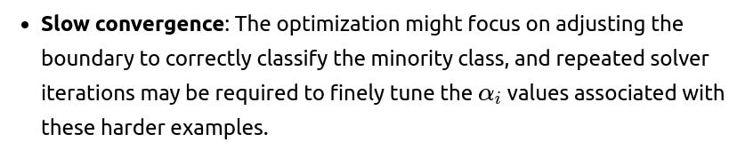
Increased number of support vectors: Frequently, minority-class points near the decision boundary all become support vectors. If the data for the majority class is also not trivially separable (in that kernel space), it can yield an even larger fraction of support vectors, which inflates the prediction-time cost.
One potential pitfall is failing to apply measures (e.g., class weighting, oversampling, undersampling) to handle imbalance. Without rebalancing the effective cost of misclassification, the model might overfit to the majority class, ironically yielding a boundary that includes more support vectors overall. This, in turn, increases the memory and computational burden.

Edge cases and real-world issues:

Reweighting or cost-sensitive SVM approaches can mitigate overfitting or underfitting but must be tuned carefully to avoid pushing the margin incorrectly.
How do multi-class extensions (like one-vs-rest or one-vs-one) impact the overall time complexity?
A standard SVM is inherently a binary classifier. For multi-class tasks with k classes, the common strategies are:
One-vs-Rest (OvR): Train k different binary SVM classifiers, each separating one class from the rest.

Impact on complexity

Inference considerations
OvR: Evaluate k decision functions at test time and pick the class with the highest (or most favorable) margin. Each decision function cost is tied to the number of support vectors for that binary classifier.

Potential pitfalls:

Memory overhead due to storing multiple SVM models.
Failing to properly tune the kernel parameters for each sub-problem can degrade performance significantly.
Edge cases:
In highly multi-class problems (like hundreds or thousands of classes), kernel SVM approaches can become computationally prohibitive, leading practitioners to prefer neural networks or tree-based methods that scale differently.
What is the role of caching strategies in modern SVM solvers, and how do they affect practical training time?

Impact on training time

If cache size is too small, frequent cache misses can degrade performance, as the solver must recompute the kernel function many times.
Pitfalls:
Memory constraints: If n is large, storing a large cache can strain system memory. A partial cache approach is used, but deciding the right cache size is non-trivial.
Dynamic scheduling: The solver might adapt which rows/columns to cache based on the frequency of access. Poorly designed caching heuristics can hamper performance.
Subtle real-world issue:

How do hyperparameter choices (like C for penalty or γ in RBF) affect the computational complexity?

Convergence behavior:
A very large C (less regularization) can create a stiffer optimization problem, where many points need to be precisely on or within the margin, potentially increasing the number of support vectors and the solver's iteration count.
A smaller C (strong regularization) may yield fewer support vectors, which can help the solver converge faster and reduce inference complexity.
Conditioning of the kernel matrix:

If γ is too small, everything can appear too similar, flattening the kernel matrix. The margin might incorrectly group many points, again increasing solver iterations.

Pitfalls and edge cases:
When γ is extremely large, or C is extremely high, you might end up with an almost “memorizing” classifier. This situation typically yields a large fraction of support vectors, ballooning memory usage, inference time, and potentially the training iteration count.

How do specialized hardware accelerators (like GPUs or TPUs) influence the training time of kernel SVMs?
While deep neural networks leverage parallelized matrix-matrix operations extensively on GPUs or TPUs, kernel SVM training does not always map as efficiently to these devices because:

Quadratic solvers: Many specialized solvers rely on data-dependent iteration flows that are less amenable to the large, dense matrix multiplications that GPUs excel at. Decomposition algorithms might sequentially pick pairs of variables to update.
Nevertheless, some acceleration is possible:
Partial GPU offloading of kernel computation or gradient calculation can reduce time, especially if the kernel function is expensive (like RBF with large d).
Pitfalls:
Transferring large amounts of data to and from the GPU can become the bottleneck.
Implementations might revert to CPU for certain steps if no efficient GPU-based factorization is available.
Edge cases:

How does feature engineering (e.g., polynomial expansions) compare to using polynomial kernels in terms of time complexity?

Real-world subtlety:
In practice, polynomial kernels are often overshadowed by the RBF kernel. Many real-world use cases prefer RBF because it handles more complex separations than a fixed polynomial degree.
If you suspect the data has polynomial interactions up to degree p, explicit expansions might be more direct for interpretability but at a potentially high computational cost.
Implementation details (like how to efficiently generate and store polynomial features) can drastically affect runtime.
How might outlier detection or robust SVM formulations affect training complexity?

Solver modifications: Some robust approaches add more constraints or turn the problem into a second-order cone program (SOCP) or require iterative reweighting. Each step might still use a kernel SVM-like solver, thereby not escaping the fundamental complexity.
Pitfalls:
Expecting that robust formulations “magically” reduce the number of support vectors or training time. While it might reduce the sensitivity to outliers, it does not necessarily reduce memory or computational overhead.
If the robust approach discards or reweights points, one must ensure that the distribution of the data is still well represented. Overzealous outlier removal can hamper generalization.
Edge cases:

Are there situations in which we can reduce kernel SVM complexity by exploiting specific data structures or geometric properties?
In some specialized scenarios, advanced data structures or geometric insights can reduce the effective complexity:
Low-rank or nearly low-rank data covariance: If the data inherently lies in a lower-dimensional manifold of dimension m≪d, or if the kernel matrix itself is nearly low-rank, methods like Nyström or incomplete Cholesky decomposition become more accurate and efficient.
Spatial data (e.g., in smaller dimensional spaces like d=2 or d=3): If the dataset is truly embedded in a low dimension, special kernel approximations or tree-based data structures (like kd-trees for approximate nearest neighbors) might accelerate certain computations, though this remains non-trivial for large n.
Special kernel structure: In some tasks (e.g., circular or spherical kernels, additive kernels), certain Fourier-based expansions or known transforms can diagonalize or partially diagonalize the kernel matrix, cutting computation time.
Pitfalls:
Such specialized approaches often require strong assumptions on data geometry. If the data does not satisfy these conditions, the method might degrade severely.
Overlooking the cost of building advanced data structures (like trees or multi-scale structures). For large n, building them might approach or exceed the naive kernel matrix building time if not carefully implemented.
Edge cases:
High-dimensional data seldom benefits from spatial partitioning.
Real-world data can be messy, invalidating many strong assumptions.
Some of these methods are highly problem-specific (e.g., certain kernel expansions only apply to shift-invariant kernels).
Can active learning or incremental learning approaches reduce the complexity for kernel SVM training?
Active learning:
The idea is to iteratively select informative samples to label from a larger unlabeled pool, thereby keeping n smaller at each training iteration. If you only label the “hard” or “uncertain” points, you might drastically reduce the training set size without sacrificing model quality.

Incremental (online) learning:
Traditional kernel SVM is not inherently online because each new data point can change the entire n×n kernel matrix. Nonetheless, specialized approaches exist to update the model with minimal re-computation (e.g., budgeted SVMs that cap the number of support vectors).
Pitfalls:

Budgeted or online approaches might severely approximate the solution, sacrificing accuracy.
Edge cases:
If your data arrives in a stream and n grows unbounded, a standard kernel SVM is infeasible. An online/budget approach is mandatory.
Active learning can achieve a smaller labeled set, but you must ensure that the unlabeled pool is large enough and that the chosen queries effectively represent the data distribution.
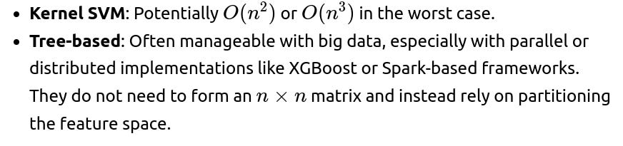
How does the time complexity of kernel SVM compare to tree-based methods (like random forests or gradient boosting) in real-world large-scale scenarios?
For large n, tree-based methods (random forests, gradient boosted decision trees) often have complexities closer to O(n log(n)) or ParseError: KaTeX parse error: Expected 'EOF', got '_' at position 33: …s \text{(number_̲of_trees)}) in practice when building balanced trees. Although each split can be O(d n log(n)) or other variations, these methods are typically more scalable and can handle larger datasets than kernel SVMs.
Differences in complexity scaling:
Pitfalls:
Overlooking that tree-based methods might have large memory usage for storing multiple trees, though it usually scales better than storing an n×n kernel matrix.

Tree-based models can also overfit if hyperparameters (like depth) are not controlled.
Edge cases:
For small-to medium-scale problems with d not huge, a kernel SVM might outperform random forests or gradient boosting on accuracy if the kernel is well-chosen.
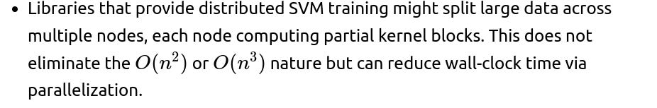
Distributed frameworks heavily favor tree-based methods at scale, while kernel SVM parallelization is more specialized.