
ML Interview Q Series: Likelihood Ratio Test: Comparing Exponential User Lifetime Rate Parameters

Browse all the Probability Interview Questions here.
5. Say you have a large amount of user data that measures the lifetime of each user. Assume you model each lifetime as an exponentially distributed random variable. What is the likelihood ratio for assessing two potential λ values, one from the null hypothesis and the other from the alternative hypothesis?
An exponential distribution with parameter λ is often used to model lifetimes or waiting times. If we have a sample of lifetimes from n users, call them x₁, x₂, ..., xₙ, and we assume each xᵢ is i.i.d. according to an exponential distribution with rate parameter λ, then the probability density function for each observation xᵢ is

When we have two competing hypotheses about the rate parameter λ (for instance, a null hypothesis λ₀ and an alternative hypothesis λ₁), we often want to assess the ratio of likelihoods under these two parameters. The likelihood function for the entire dataset {x₁, x₂, ..., xₙ} under a particular λ is

The likelihood ratio for comparing λ₀ (null) against λ₁ (alternative) is defined as
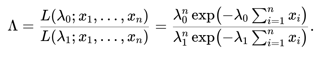
Simplifying, this becomes

This ratio forms the core of the likelihood ratio test: we compare this ratio (or its logarithm) to a threshold in order to decide whether to favor the null hypothesis (λ₀) or the alternative hypothesis (λ₁).
In extremely detailed form, here is how we arrive at it step by step:
• Each observation xᵢ has exponential PDF λ e^(-λ xᵢ). • Because the data points are assumed i.i.d., we multiply the PDF for each observation to get the joint likelihood. • For hypothesis H₀: λ = λ₀, the likelihood is λ₀^n e^(-λ₀ Σxᵢ). • For hypothesis H₁: λ = λ₁, the likelihood is λ₁^n e^(-λ₁ Σxᵢ). • The likelihood ratio is the fraction of these two likelihoods.
Hence, the direct answer to the question “What is the likelihood ratio for assessing two potential λ values?” is exactly

Likelihood Ratio Test In Practice The likelihood ratio test (LRT) typically uses a decision rule of the form: reject H₀ if Λ < c (where c is chosen based on a significance level α). Often, we look at the log-likelihood ratio

and compare it to a threshold that is derived from statistical theory (for instance, using the asymptotic χ² distribution for the log-likelihood ratio under certain regularity conditions).
To illustrate how we might compute this in code given a collection of user lifetimes, we can do something like:
import numpy as np

def likelihood_ratio(data, lambda0, lambda1):
    # data is an array of user lifetimes
    n = len(data)
    sum_of_data = np.sum(data)

    # Compute numerator: L(lambda0)
    L0 = (lambda0**n) * np.exp(-lambda0 * sum_of_data)

    # Compute denominator: L(lambda1)
    L1 = (lambda1**n) * np.exp(-lambda1 * sum_of_data)

    return L0 / L1

# Example usage:
data_samples = np.array([2.3, 1.1, 0.7, 3.5, 4.2])  # Example lifetimes
lambda0 = 0.5
lambda1 = 0.8
lr_value = likelihood_ratio(data_samples, lambda0, lambda1)
print("Likelihood Ratio:", lr_value)
This code gives the ratio directly. From there, one would typically compare log(lr_value) to some threshold that is derived for the test, or equivalently compare lr_value itself to some threshold.
What If the Data Is Not Truly Exponential?
One immediate follow-up question is what happens if the data is not actually exponentially distributed in reality. In real-world scenarios, user lifetimes can have more complicated distributions (for example, Weibull, Gamma, or even a mixture of distributions). The exponential distribution assumes a constant hazard rate, but real user retention can have different hazard rates over time. If this assumption is violated, the model can be misspecified, and the likelihood ratio test for distinguishing λ₀ from λ₁ can lose power or can be invalid.
In practice, analysts might use goodness-of-fit tests, or cross-validate with alternative distributions to confirm that the exponential assumption is not severely violated. Another approach could be to apply a parametric survival analysis method with a more flexible distribution. Alternatively, one might take a non-parametric approach if there is enough data.
How Do We Derive a Confidence Interval for λ?
Another likely follow-up is about obtaining confidence intervals for the rate parameter. In the exponential distribution, the Maximum Likelihood Estimate (MLE) for λ is
One can use asymptotic properties: since the MLE is asymptotically normal with variance that can be approximated by the inverse of the Fisher information, we can derive approximate confidence intervals. Specifically, the Fisher information for λ in the exponential distribution, based on n i.i.d. samples, is

Thus, the asymptotic variance of the MLE is λ² / n, and an approximate confidence interval is

where zᵅ/₂ is the (1−α/2) quantile of the standard normal distribution. More exact methods also exist (inversion of the likelihood ratio test itself, for instance).
How Does This Compare to a Bayesian Approach?
Another tricky follow-up is how the likelihood ratio test compares to Bayesian methods. In a Bayesian framework, you would incorporate prior distributions on λ and compute posterior distributions given the data. Instead of forming a ratio of likelihoods alone, you would typically compare the posterior probabilities of H₀ vs. H₁ (or compute the Bayes factor, which is the ratio of marginal likelihoods). The results can be similar if non-informative priors are used, but the Bayesian approach can incorporate more prior knowledge about λ and produce different thresholds.
What Happens If the Data Is Censored?
In some user lifetime studies, not all users have “exited” the system by the time of analysis. This leads to right-censored data (for example, a user who joined 10 days ago and is still active has only a partial lifetime observation). In an exponential model, the likelihood contribution for a user who is still active after time t is the survival function e^(-λ t). The likelihood ratio test still works, but you must adapt the likelihood appropriately to include these survival function terms for censored observations:

where yⱼ are the censoring times (i.e., the time up to which you have observed the user without an exit event). The ratio is then formed in the same manner, plugging in λ₀ and λ₁ for the complete and censored observations. Real-world user lifetimes are often censored, so it’s crucial to account for it properly when forming a hypothesis test for λ.
Finding the MLE for λ and Performing the LRT
Sometimes, another follow-up question is about how the test statistic is formed for the final decision. After forming the likelihood ratio, we typically compute the test statistic

where Λ is the ratio of the maximum likelihood under H₀ to the maximum likelihood under H₁ (or vice versa, depending on your testing convention). Under usual regularity conditions and large n, this statistic approximately follows a χ² distribution with degrees of freedom equal to the difference in the number of parameters between H₀ and H₁ (in this case, typically 1 if the only difference is λ). We then compare it to critical values from the χ² distribution or compute a p-value.
If −2 ln(Λ) is large enough, this indicates the alternative hypothesis H₁ is favored. This approach is fundamental to many parametric hypothesis tests in statistics.
Python Code Example for Fitting and Testing
Another angle might be a practical step-by-step code snippet that:
Reads in the data.
Fits the MLE for λ (although in the question we assume λ₀ and λ₁ are already specified, for a test scenario).
Computes the likelihood ratio.
Returns the test statistic and a p-value.
Here is a more extended approach:
import numpy as np
from scipy.stats import chi2

def exponential_log_likelihood(data, lam):
    n = len(data)
    return n * np.log(lam) - lam * np.sum(data)

def lrt_exponential(data, lambda_null, alpha=0.05):
    # log-likelihood under null (fixed lambda_null)
    ll_null = exponential_log_likelihood(data, lambda_null)

    # MLE for lambda under alternative
    n = len(data)
    sum_of_data = np.sum(data)
    lambda_mle = n / sum_of_data

    # log-likelihood under alternative
    ll_alternative = exponential_log_likelihood(data, lambda_mle)

    # Likelihood ratio statistic
    test_stat = -2 * (ll_null - ll_alternative)

    # Under large n, test_stat ~ chi-square with df=1 (since only 1 extra parameter in alternative)
    p_value = 1 - chi2.cdf(test_stat, df=1)

    reject = (p_value < alpha)
    return test_stat, p_value, reject

# Example usage:
data_samples = np.array([2.3, 1.1, 0.7, 3.5, 4.2])  # example lifetimes
lambda0 = 0.5

ts, pval, decision = lrt_exponential(data_samples, lambda0, alpha=0.05)
print("Test Statistic:", ts)
print("p-value:", pval)
print("Reject H0?", decision)
While the question specifically asked for the ratio of the likelihoods at λ₀ vs. λ₁, in real usage you might want to compare λ₀ (or an entire family of potential null values) to the MLE-based alternative or do a full parametric test. This is a typical pattern in parametric hypothesis testing for the exponential distribution.
Practical Concerns and Edge Cases
In large-scale user data, edge cases to watch out for include:
• Extremely large or small user lifetimes that might push the rate estimates (and thus the exponent terms) to numerically underflow or overflow. Log-transforming the likelihood (log-likelihood) is a standard way to handle this. • Many zero or near-zero lifetimes if the system logs user churn extremely quickly. Some robust approaches or slight data cleaning might be necessary. • Missing or partially observed data: as discussed, for right-censored data or other forms of incomplete observation, the likelihood ratio must incorporate the survival component for unobserved lifetimes beyond the last known time point.
Recap
The concise mathematical ratio for comparing two specific λ values, λ₀ vs. λ₁, using a dataset of n i.i.d. exponential samples x₁, x₂, …, xₙ is:

However, the deeper understanding involves how to use this ratio in hypothesis testing, how to interpret the result, and how to adapt to real-world complications such as non-exponential data or censoring.
This forms the foundation for parametric hypothesis testing with the exponential distribution, and the same approach extends to many other distributions where the ratio of likelihoods can be computed in a closed-form expression.
Below are additional follow-up questions
How does the memoryless property of the exponential distribution affect our interpretation of user lifetimes, and what pitfalls might arise if lifetimes are not truly memoryless?
The exponential distribution is unique among continuous distributions for having the memoryless property. This means that no matter how long a user has already stayed, the probability they leave in the next interval remains the same. In notation, for an exponential random variable X with rate λ,

In the context of user lifetimes, this implies that a user who has remained in the system for a certain duration does not have any lower or higher probability to churn in the next instant compared to a new user.
Potential pitfalls
Non-constant hazard: Real-world churn often depends on user tenure: a user might be more likely to churn early on, then less likely after they pass some milestone. This violates the memoryless property. If we rely on the exponential assumption, we can underestimate or overestimate the churn rate for different user subpopulations.
Ignoring user behavior changes: If the hazard rate changes over time (e.g., after onboarding, the user is more “sticky”), then an exponential model (with constant λ) might fit poorly. The likelihood ratio test comparing two exponential rates might still be mathematically valid but might not capture the real shape of user retention.
Misleading test outcomes: Even if the test indicates a better fit for one λ vs. another, it does not prove the data truly follows an exponential distribution. A better approach could be to test the exponential assumption directly (e.g., with goodness-of-fit tests or survival curve checks) before performing the likelihood ratio test for specific rate parameters.
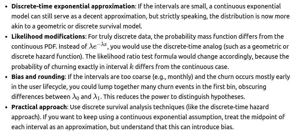
If we only have aggregated or discretized time intervals for churn data, how does that change the testing procedure?
In many real-world applications, user lifetimes are not observed with exact continuous timestamps. Instead, data might be summarized in daily or weekly aggregates (for instance, “user churned in the 2nd week,” or “user was active through week 5, then churned in week 6”). This effectively discretizes what was originally a continuous process.
Testing considerations
What if the user population is heterogeneous, consisting of subgroups that have different churn rates?
A single exponential parameter λ implies a homogeneous population with the same churn rate. In practice, some users may churn quickly while others rarely churn, suggesting multiple underlying distributions or a mixture model.
Implications

Can the likelihood ratio test be used in an online or sequential testing scenario, where data arrives continuously over time?
Yes. In online or sequential testing, you collect user data in real time and want to update your hypothesis test as new lifetimes are observed.
Key considerations
Sequential test design: Classical hypothesis tests assume a fixed sample size. When data arrives continuously, using the standard LRT at arbitrary stopping points can inflate Type I error rates. Specially designed sequential tests (e.g., Sequential Probability Ratio Test or “SPRT”) maintain error rate control.
SPRT approach: The SPRT accumulates log-likelihood ratios as data arrives. As soon as the ratio crosses an upper or lower threshold, you make a decision (accept or reject the null). If it remains in an inconclusive region, you keep collecting more data.
Pitfalls:
If you do repeated peeking at the data without adjusting thresholds, you can erroneously reject or fail to reject H₀ more often than expected under the nominal α level.
Once you incorporate the user lifetimes in an online fashion, partial observations (censored data) are more common. The test must account for the fact that some users who started more recently have not yet churned.


How can we incorporate user-level covariates (e.g., demographics, usage patterns) into the exponential model and the likelihood ratio test?
When user churn depends on additional features, a simple exponential distribution with a single rate λ may be too restrictive. Instead, we can employ parametric survival models that allow λ to vary based on covariates. One popular approach is to log-transform the rate:

Likelihood ratio testing
Interpretation: A statistically significant result could mean that adding certain covariates significantly improves the fit, indicating those features are relevant for explaining churn variation.
Pitfalls:
Overfitting if you include too many covariates with limited data.
Multicollinearity if the covariates are highly correlated. This can make coefficient estimates unstable and complicates the interpretation.
Violations of model assumptions if the relationship between log(λ) and covariates is not linear.
How do we handle extremely large datasets and ensure computational efficiency when calculating the likelihood ratio?
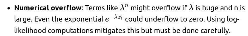
In large-scale ML or data engineering environments, user lifetime datasets can have millions or billions of records. The naive approach of directly multiplying large exponentials or raising λ to a huge power can lead to numerical underflow or overflow.
Strategies
Log-likelihoods: Compute sums of log probabilities instead of directly computing products. This is standard practice:

Vectorized operations: Libraries like NumPy or PyTorch handle large arrays efficiently on CPUs or GPUs, but you should keep memory constraints in mind. Summations need to be carefully done to avoid numeric instability (e.g., using double precision or appropriate summation algorithms).
Distributed systems: For extremely large data, you might distribute the log-likelihood computation across multiple machines, summing partial results. The final ratio is then straightforward to compute once each node sends back its partial sum of lifetimes and count of records.
Pitfalls:

Communication overhead in distributed settings if you frequently update partial sums. A well-batched approach reduces overhead.
If λ is extremely large or extremely small, what numerical issues or misinterpretations can arise?
When λ is very large, this implies users typically churn very quickly (short lifetimes). Conversely, a very small λ suggests extremely long retention. Both extremes can cause complications:
Large λ

Model misfit: If λ is large, small variations in data can drastically change the likelihood. This can cause the LRT to be sensitive if the data truly does not support such a high rate.

Small λ

Misinterpretation: A tiny λ may indicate a near-zero churn rate. You must confirm that data genuinely suggests near-permanent user retention, or if instead your model is incorrectly capturing just a subset of the population.
How do we address partial lifetimes or “delayed entry” scenarios where some users started before the observation period or only part of their usage history is available?
Besides right-censoring (users who have not yet churned), there are other complexities in real user data:
Left-truncation or delayed entry: Some users might have joined the system before your observation window started. You only begin tracking them mid-lifetime. Standard exponential modeling would incorrectly treat their “start” as time 0, ignoring the fact that they already “survived” up to that point.
Intermittent observation: Some lifetimes might have gaps in observation. For instance, a user might go inactive for a while, then come back. Determining the moment of “churn” is ambiguous.
Adapting the likelihood
For left-truncation, the correct term for a user who enters the study at time a and churns at time b>a is proportional to:


For intermittent observation, you need a carefully defined event time or a well-defined censoring rule.
Pitfalls:
Mixing partial lifetimes with full lifetimes without adjusting the likelihood can bias the rate estimate, often leading to underestimation or overestimation of churn depending on the distribution of entry times.
Dropping partially observed users is a common but naive approach that loses data and can bias results toward more engaged or long-lived users.
If we suspect the system changes over time (non-stationarity), does a single λ still make sense, and how can we test that?
Systems can evolve: for example, the product might have improved features that affect churn rates in later cohorts, or external events might change user behavior. A single λ across the entire data history may no longer be appropriate.
Approaches to handle time-varying behavior

Time-dependent covariates: In parametric survival models, you can incorporate “calendar time” or “cohort effects” as a covariate in λ. This allows the rate to systematically shift over time.
Moving window analysis: Instead of using all historical data at once, you apply the exponential fit to rolling windows or cohorts, then see if the best-fit λ changes. If it does, that’s evidence of non-stationarity.
Pitfalls
If the system truly changes frequently, forcing a single λ can mask significant shifts in user retention patterns. A test that lumps together old data with new data can be misleading about current churn rates.
Over-segmentation can reduce data within each segment, causing high variance in rate estimates.
How do we interpret Type I and Type II errors in the context of a likelihood ratio test for user churn rates?
