ML Interview Q Series: Linear Regression: Equivalence of Maximum Likelihood and Minimum Squared Residuals with Gaussian Errors.

Browse all the Probability Interview Questions here.

19. Suppose you are running a linear regression and model the error terms as normally distributed. Show that maximizing the likelihood of the data is equivalent to minimizing the sum of squared residuals.

Understanding the Relationship Between Likelihood and Sum of Squared Residuals in Linear Regression

It helps to start with a linear regression framework where each observed response value is modeled as a linear function of the predictors plus a noise term. Let the observations be denoted by pairs

for

i=1,…,n

. The vector of predictor variables for the i-th observation is

, and the corresponding scalar response is

. We assume a linear model of the form

where

are the unknown parameters and

are error terms. If we assume these error terms are independent and normally distributed with zero mean and variance

, we can write

This assumption about normality will motivate the link between maximizing the likelihood of the data and minimizing the sum of squared residuals.

Likelihood of the Observed Data Under Gaussian Assumptions

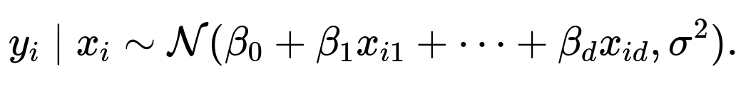
When errors are normally distributed, each observation

given its predictors

and the parameters

β

is distributed as

Hence, the probability density for a single observation

can be written as

where

is understood to include a leading 1 if we fold

into the parameter vector

β

for notational simplicity.

Since the observations are assumed independent, the joint likelihood of all data points

given

can be written as the product of these individual densities:

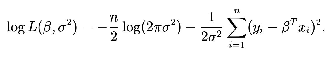
To make it simpler, we often consider the log of the likelihood, which is called the log-likelihood:

We can split this into two separate parts:

Maximizing the Log-Likelihood with Respect to

β

To find the parameter vector

β

that maximizes the log-likelihood, we note that the first term depends on

but not on

β

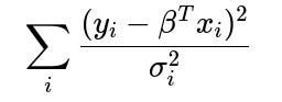
, while the second term depends on both. However, for a fixed

, maximizing the log-likelihood with respect to

β

is equivalent to minimizing

That sum is precisely the sum of squared residuals. Therefore, under the Gaussian noise assumption, the maximum likelihood estimate of

β

is the same as the parameter choice that minimizes the sum of squared residuals. This equivalence is why Ordinary Least Squares (OLS) emerges naturally from the normality assumption on the errors.

Mathematically, the partial derivative of the log-likelihood with respect to

β

(for fixed

) leads to the normal equations, which in matrix form can be written as

Solving these yields the ordinary least squares solution

which is also the solution to minimizing the sum of squared errors in linear regression. Thus, maximizing the likelihood under Gaussian errors is exactly the same as minimizing the sum of squared deviations from the regression hyperplane.

Implementation Example in Python

Below is a simple code snippet using NumPy that illustrates how one might solve for the least squares estimate. In practice, frameworks like scikit-learn, PyTorch, or TensorFlow typically provide efficient built-in routines for this purpose, but this code shows the basic idea.

import numpy as np

# Suppose X is an n x d matrix (including a column of ones for intercept)
# Suppose y is an n x 1 vector of targets

# Generate a random dataset for illustration
np.random.seed(42)
n, d = 100, 2  # 100 samples, 2 features (the first feature will be all ones for the intercept)
X = np.ones((n, d))
X[:, 1] = np.random.randn(n)
true_beta = np.array([1.5, -2.0])  # intercept = 1.5, slope = -2.0
noise = 0.5 * np.random.randn(n)
y = X.dot(true_beta) + noise

# Solve for beta using the OLS closed-form solution
beta_est = np.linalg.inv(X.T.dot(X)).dot(X.T).dot(y)

print("True beta:", true_beta)
print("Estimated beta:", beta_est)

This code sets up a design matrix X with one feature plus an intercept term, simulates target values with an added normal noise, and solves for the linear regression parameters using the closed-form Ordinary Least Squares solution. The method finds the parameter values that minimize the sum of squared residuals, which is the same parameter choice that maximizes the likelihood when the errors are assumed to be normally distributed.

What if the Error Distribution is Not Gaussian?

If the noise distribution is not Gaussian, maximizing the likelihood no longer corresponds exactly to minimizing the sum of squared errors. For instance, if you assume a Laplace distribution for the error terms, maximizing the likelihood becomes equivalent to minimizing the sum of absolute errors. This is the connection between model assumptions and the corresponding cost function you are minimizing.

Could We Derive the Same Result by Minimizing the Negative Log-Likelihood?

Yes, minimizing the negative log-likelihood of a Gaussian model is the same as maximizing the log-likelihood. The negative log-likelihood for a Gaussian model is proportional to the sum of squared residuals plus terms that do not depend on

β

, so minimizing that expression in

β

also yields the classical Ordinary Least Squares solution.

Why Do We Often Use the Log-Likelihood Instead of the Likelihood?

The likelihood can be a product of many small numbers (probability densities) multiplied together, which can become numerically unstable or extremely small. Taking the log transforms the products into sums and typically leads to more numerically stable computations. It also turns exponential functions into linear forms that are easier to differentiate and optimize.

How Does This Relate to Gradient-Based Methods in Deep Learning?

Although the classical linear regression solution can be found in closed form, modern deep learning often uses gradient-based optimization (like stochastic gradient descent) to handle much more complex models without closed-form solutions. Even for linear regression, you can still arrive at the same result (minimizing the sum of squared residuals) by applying gradient descent to the mean squared error (MSE) cost function, which again parallels maximizing the Gaussian log-likelihood.

Potential Pitfalls and Edge Cases

In practical scenarios, the assumption of normal errors might be only approximately valid. If errors have outliers or heavy tails, the sum of squared residuals can yield parameter estimates heavily influenced by extreme data points. Additionally, if features in the design matrix are highly correlated, the matrix

may be close to singular, causing instability in the closed-form solution. Regularization techniques like ridge regression or lasso can help in such cases, effectively modifying the likelihood or the cost function to include constraints or penalties on the parameter magnitudes.

Follow-up Question 1

Why does the maximum likelihood approach under a Gaussian assumption lead to the same solution as Ordinary Least Squares, but under a Laplacian assumption it leads to Least Absolute Deviations?

When errors follow a Gaussian distribution, the probability density is proportional to the exponential of the squared error. This makes the log-likelihood function proportional to the sum of squared errors, so minimizing that sum (or maximizing the likelihood) yields the same parameter estimates. On the other hand, for Laplace-distributed errors, the density is proportional to the exponential of the absolute error. Taking the log then leads to minimizing the sum of absolute deviations. This shows how the choice of error distribution in a probabilistic model directly affects the form of the objective function we minimize.

Follow-up Question 2

How do we interpret the variance

in the context of maximizing the likelihood?

In this Gaussian regression setting,

represents the variance of the noise or the error term. When you maximize the likelihood with respect to

(once

β

is found), you can solve for the variance that best explains the residuals in the data. Specifically, one can show that the maximum likelihood estimate of

is the average of the squared residuals. This links neatly to the idea that the residuals have variance

if the model is correctly specified.

Follow-up Question 3

If the design matrix is not full rank, how does that affect the maximum likelihood estimate?

If the matrix

is not invertible (or very close to being singular), this indicates a collinearity or linear dependence among some features. The closed-form solution for

β

becomes either not uniquely determined or numerically unstable. In this situation, infinite sets of solutions can all minimize the sum of squared errors equally well, making the maximum likelihood estimate non-unique. Practitioners address this by using regularization (like ridge regression), which modifies the objective by adding a penalty term and ensures that the matrix to be inverted remains well-conditioned.

Follow-up Question 4

Can you show a simple gradient-based derivation that arrives at the same result?

Yes, one can start with the mean squared error cost function, which is proportional to the sum of squared residuals, and take its gradient with respect to

β

. If we arrange our data in matrix form so that

y

is an

n

-dimensional vector of targets and

X

is the

n×d

design matrix (including a column of 1s for the intercept), the cost function can be written as

Taking the gradient and setting it to zero yields

which leads to

whose solution is

This matches precisely the solution obtained by maximizing the Gaussian log-likelihood.

Follow-up Question 5

Why might we prefer iterative (like gradient descent) or approximate methods over the closed-form solution in modern machine learning?

In high-dimensional or large-scale problems, computing

directly becomes impractical or very memory-intensive. Iterative methods such as gradient descent or stochastic gradient descent can handle extremely large datasets and high-dimensional parameter spaces without needing to invert large matrices explicitly. Moreover, in deep learning, the model structures are far more complex and cannot be expressed in a neat closed-form solution. Hence, gradient-based methods are the go-to solution in most real-world scenarios, even though for standard linear regression the closed-form solution theoretically exists.

Follow-up Question 6

Are there any assumptions about independence of errors, and how crucial is that assumption?

Yes, classical linear regression generally assumes that each error term

is independent of the others and identically distributed. This independence underpins the factorization of the likelihood into the product of individual densities. If errors are correlated (as in time-series data with autocorrelated residuals), standard linear regression methods can be suboptimal or yield incorrect confidence intervals and significance tests. In such scenarios, one might switch to models specifically designed for correlated errors, such as Generalized Least Squares or methods that incorporate correlation structures in the noise model.

---

Below are additional follow-up questions

How does the choice of loss function influence the sensitivity to outliers, and are there variants of Gaussian-based regression that are more robust?

When we assume Gaussian noise, the log-likelihood expression becomes proportional to the sum of squared residuals. Squaring the residuals magnifies large errors more than smaller ones, causing outliers (points that deviate substantially from the rest) to have a significant influence on the resulting parameter estimates. In real-world data, these outliers could arise due to measurement errors or unusual, rare phenomena, and their presence may unduly distort the regression model.

To mitigate this, researchers sometimes adopt robust regression techniques. One common approach is to replace the standard Gaussian assumption (leading to squared residuals) with distributions less sensitive to large deviations. For instance, a robust alternative is to place a heavier-tailed distributional assumption on the error term (e.g., a Student’s t-distribution). The t-distribution with a smaller degrees-of-freedom parameter has heavier tails than a Gaussian, reducing the impact of outliers on the parameter estimates. Another strategy is to use an iterative reweighting of residuals, such as in M-estimators, which reduce the contribution of points deemed outliers.

Potential pitfalls include choosing a too heavy-tailed distribution, leading to insufficient penalization of moderate errors. Also, iterative robust methods may converge more slowly or get stuck if the initial guesses or step sizes are poorly chosen. In practice, it is essential to balance outlier resilience with stable convergence and interpretability.

What happens if we do not include an intercept term in our model, and how does that affect the maximum likelihood estimation?

Including an intercept (often represented in the design matrix by a column of ones) allows the regression hyperplane to shift up or down relative to the axes. If no intercept is included, the hyperplane is forced to go through the origin. The implications for maximum likelihood are as follows:

1. If the true relationship between features and targets does not pass through the origin, then omitting the intercept introduces a systematic bias in the model. The estimate of parameters will attempt to account for this by adjusting slopes in a way that might lead to higher residual variance.

2. The variance estimate

   

   in a model without intercept may be artificially inflated, because residuals will systematically deviate from zero if the relationship does not naturally pass through the origin.

3. In terms of maximum likelihood, the log-likelihood function is still defined (under the Gaussian assumption) using the sum of squared residuals, but the residuals themselves can be systematically larger due to the forced through-origin constraint. This typically results in a suboptimal fit if a non-zero intercept is appropriate.

A possible edge case is a dataset known to pass through the origin (e.g., physical laws that dictate zero input leads to zero output). In that special case, omitting the intercept can be correct and might reduce the risk of overfitting the constant term. However, in most real-world contexts, the intercept is crucial.

How can we formally verify that the maximum likelihood estimates for linear regression are unbiased estimators of the true parameters?

Under the classical assumptions—namely that the design matrix is full rank, errors are independent and identically distributed as

, and the model is correct (i.e., linear structure plus Gaussian noise)—we can show that the expected value of the Ordinary Least Squares (OLS) estimator equals the true parameter vector. The derivation hinges on:

1. The OLS solution being

   

   2. Given

   

   we have

   

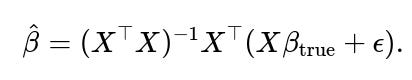
3. The expectation of

is

4. Assuming

and

X

is non-random (or treated as fixed in the classical sense),

Hence, the estimator is unbiased. Subtle issues arise when the design matrix or the error distribution violates the standard assumptions (e.g., non-zero mean errors or random features correlated with errors). In practice, data might not perfectly follow these rules, which can make the OLS estimator biased or inconsistent. That is why domain checks and robust modeling assumptions are often required.

How do we address the scenario when data is missing or partially observed, and how does it affect the maximum likelihood approach?

In real-world contexts, it is not uncommon for some observations to be incomplete, with missing feature values or target values. Naively ignoring these incomplete rows can reduce sample size, weakening statistical power. Depending on the missingness mechanism (Missing Completely at Random, Missing at Random, or Missing Not at Random), different approaches exist:

1. Listwise Deletion: Drop all rows with missing data. This simplifies the likelihood but may introduce bias if the data is not missing completely at random.

2. Imputation Methods: Attempt to estimate or “fill in” missing values. For example:

   • Simple methods (mean imputation, median imputation) can bias variance estimates or reduce data variability.

   • More advanced approaches (multiple imputation, regression-based imputation) better incorporate uncertainty and relationship with other features.

3. Expectation-Maximization (EM): An iterative maximum likelihood technique that treats missing data as latent variables. The algorithm alternates between estimating the missing values based on current parameter estimates (E-step) and updating the parameters to maximize the likelihood (M-step).

The EM algorithm is particularly relevant to linear regression under a Gaussian assumption, as each step often has closed-form updates. However, it can be computationally heavier and can converge to local optima if not carefully initialized or if the data deviate from the normal assumption. Moreover, the presence of missing data can exacerbate identification problems (e.g., collinearity), so practitioners need to watch out for ill-conditioned updates.

How do we handle a situation where the noise variance

is not constant but depends on the predictors or the true mean (heteroscedasticity)?

Heteroscedasticity means that the variance of the error term is not uniform across all observations; instead, it may depend on certain predictor values or predicted responses. This violates the classical homoscedasticity assumption used in deriving the Ordinary Least Squares (OLS) solution as the Best Linear Unbiased Estimator (BLUE).

In such scenarios, maximizing the standard Gaussian likelihood is no longer optimal, because the assumption

is replaced with something like

, where

varies among observations. One approach is:

1. Weighted Least Squares (WLS): If we know or can estimate

   

, we can incorporate weights in the objective function. The negative log-likelihood then becomes proportional to

, assigning higher weight to observations with smaller variance.

1. Generalized Least Squares (GLS): A more general framework for correlated and/or heteroscedastic errors. One posits a covariance structure

   Σ

   for the error terms and then uses that in place of

   

   in the classical derivations.

Potential pitfalls include:

• Inaccurate variance modeling: If the user incorrectly specifies

  

  or the structure of

  Σ
  , the resulting estimates might be worse than naive OLS.

• Computational Complexity: Estimating a full covariance structure can be expensive for large datasets.

When performing linear regression in high-dimensional spaces (e.g., more features than samples), how does this affect the maximum likelihood solution?

In a high-dimensional setup—often referred to as the “p >> n” scenario—the matrix

becomes singular or nearly singular, meaning the ordinary least squares closed-form solution is not uniquely defined. Several implications arise:

1. Overfitting: With many parameters and few data points, the model can fit noise rather than the underlying signal.

2. Non-unique MLE: There can be infinitely many parameter vectors that yield the same minimized sum of squared residuals, making standard OLS ill-defined in a practical sense.

3. Regularization: Approaches like ridge regression (L2 penalty) or lasso (L1 penalty) impose constraints on the parameter space, leading to more stable estimates. These can be viewed as penalized maximum likelihood approaches under specific prior assumptions (e.g., Gaussian prior for ridge, Laplacian prior for lasso).

Edge cases happen if even with regularization, certain features are perfectly collinear or extremely correlated. The solution might still be unstable. Proper cross-validation and dimensionality reduction (like PCA or domain-driven feature selection) often become essential.

What if the residuals are not identically distributed, even if they are individually Gaussian? For instance, if each data point has a different variance or a different mean structure?

Non-identical distributions break the simple i.i.d. assumption. Even if each error is Gaussian, the model’s structural assumptions might fail if the mean function or the variance structure changes per observation. The classical OLS objective is derived from the assumption

If the variance

is not constant or if the mean depends on other factors not captured by

, then maximizing the standard Gaussian likelihood is no longer the correct approach. Instead, you might:

1. Use Weighted Least Squares if the variance changes per data point but remains known or estimable.

2. Use Generalized Linear Models (GLMs) with appropriate link and variance functions if the mean-variance relationship is more complex (e.g., for count data or binary data).

Pitfalls include a mismatch between the chosen model family and the actual data. Even if you forcibly apply OLS, your inferences on confidence intervals and significance may be misleading.

How do we reconcile maximum likelihood approaches with Bayesian inference in linear regression?

From a Bayesian perspective, you place a prior distribution on the parameters (e.g., a Gaussian prior for each coefficient) and then update to a posterior distribution based on the likelihood of observed data. This means:

• The classical maximum likelihood estimate (MLE) is a single point in the parameter space that maximizes the likelihood.

• Under a Bayesian approach, you compute the posterior, which is proportional to the product of the prior and the likelihood. The maximum a posteriori (MAP) estimate is then the parameter vector that maximizes the posterior distribution.

For linear regression under a Gaussian prior, the MAP estimate often coincides with ridge regression. It can also be shown that if you assume a Laplace prior on parameters, the MAP estimate coincides with lasso. Real-world issues include the choice of prior: a poor choice can skew results. Also, exact Bayesian computations might require integration over large parameter spaces, typically handled via Markov Chain Monte Carlo (MCMC) or variational methods in practice.

How does collinearity between predictors influence the maximum likelihood estimator in linear regression, and what are some best practices to diagnose and address collinearity?

Collinearity arises when two or more predictors are (almost) linearly dependent. For example, if one predictor is a near-scaled version of another. This leads to:

1. Instability of Estimates: Small changes in the data can produce large variations in parameter estimates. The matrix

may be close to singular, making

numerically unstable.

2. Inflated Variance of Coefficients: Collinear predictors can cause large standard errors for parameter estimates, complicating interpretability.

Diagnosing collinearity can be done via:

• Variance Inflation Factor (VIF): A high VIF indicates that a predictor is highly correlated with other predictors.

• Condition Number of

• : A large condition number implies near-singular behavior.

Addressing collinearity involves:

• Removing or combining redundant features if domain knowledge indicates they provide overlapping information.

• Applying dimensionality reduction, such as PCA, to compress correlated features into fewer components.

• Regularization (ridge regression) which penalizes large coefficients and stabilizes the inversion.

A subtle trap is that collinearity might not be obvious if the correlation matrix does not reveal a single pair of highly correlated variables but multiple partial correlations among groups of variables. Always validate the design matrix thoroughly.

In what ways does linear regression with maximum likelihood assumptions differ from generalized linear regression approaches, such as logistic or Poisson regression?

While linear regression under Gaussian assumptions leads to a sum-of-squares cost function, generalized linear models (GLMs) adapt the distribution (and corresponding link function) to the nature of the response variable:

1. Logistic Regression: For binary outcomes, the Bernoulli distribution is used, and the logit link is employed. The negative log-likelihood becomes the cross-entropy or logistic loss, not the sum of squares.

2. Poisson Regression: For count data, errors are modeled via a Poisson distribution, and the link is typically the log function. The cost function or deviance differs from the sum of squares.

Although the principle of maximum likelihood remains consistent—choosing parameters that maximize the likelihood of observed data—the resulting objective functions differ because each distribution dictates a different form for the log-likelihood. Pitfalls include using the wrong distribution or ignoring overdispersion (variance higher than the mean) in count data, which might degrade the fidelity of maximum likelihood estimates.

How do non-linear transformations of predictors or polynomial expansions affect the underlying assumption of Gaussian errors?

When we introduce polynomial or non-linear transformations of predictors, the model form becomes:

where

could be, for example, a polynomial expansion or other non-linear transformation. As long as the error term

remains normally distributed with constant variance around the mean function

the maximum likelihood approach under that Gaussian assumption still leads to minimizing squared residuals between

and

However, potential complications arise:

1. Overfitting: High-degree polynomial expansions can fit noise and lead to poor generalization.

2. Collinearity Within Polynomial Terms: Terms like

and

can be correlated with each other and with the original

exacerbating collinearity.

3. Non-constant Variance: Sometimes, the polynomial or non-linear transformation might inadvertently make the error variance grow with larger

1. values. This violates the constant-variance assumption.

For robust inference, one might use transformations or weighting schemes to stabilize variance, or might rely on cross-validation to choose the model complexity that best balances fit and generalizability.

Can we use maximum likelihood estimation in linear regression to compute confidence intervals or prediction intervals, and what assumptions are needed?

Yes, after fitting a linear regression via OLS (which coincides with the MLE under Gaussian assumptions), we typically compute:

1. Confidence Intervals for Parameters: Based on the estimated variance-covariance matrix of

   

   If the errors are Gaussian and independent,

   

   follows a multivariate normal distribution, and each parameter can be given a confidence interval using the appropriate t-distribution or normal approximation (when sample size is large).

2. Prediction Intervals: Combining the uncertainty in

   

   plus the residual variance

   

   to express the uncertainty in a new prediction.

Pitfalls:

• If the errors are not Gaussian or independent, standard confidence and prediction intervals may be inaccurate.

• Heteroscedasticity invalidates the straightforward usage of

  σ2(X⊤X)−1.

  

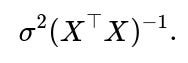
• Correlation between errors (e.g., in time-series) can shrink or inflate interval widths unpredictably if not accounted for in the covariance structure.

Under what circumstances do iterative reweighted least squares (IRLS) methods become relevant for maximum likelihood estimation in regression, and how does IRLS differ from standard OLS?

Iterative Reweighted Least Squares (IRLS) methods emerge when:

• The objective function arises from a likelihood that is not strictly the sum of squared errors but can be turned into a weighted least squares form at each iteration. This is common in generalized linear models, including logistic and Poisson regression.

• Robust regression frameworks (like Huber loss or Tukey’s biweight) use IRLS to down-weight outliers in each iteration.

The high-level distinction from standard OLS is that in IRLS, at each iteration, we compute updated weights based on the current residuals or model predictions, forming a weighted least squares problem. That is solved for the new estimates of parameters, and then the process repeats. By contrast, standard OLS (for linear Gaussian models) has a single closed-form solution and needs no iterative refinement.

Potential pitfalls include divergence or oscillatory behavior if the iteration is not well-tuned, especially when the data is particularly noisy or the model is highly nonlinear. Careful step-size selection or damping can be necessary.

How can diagnostic tests like the Shapiro-Wilk test for normality of residuals or Q–Q plots help validate the maximum likelihood assumptions of linear regression?

A core assumption in classical linear regression is that the errors are normally distributed. While the MLE under a Gaussian assumption is still the solution that minimizes sum of squared residuals regardless, the standard inferences and confidence intervals rely heavily on this normality assumption (and on homoscedasticity).

1. Shapiro-Wilk Test: A formal statistical test that checks if your residuals deviate significantly from a normal distribution. A low p-value suggests non-normality, potentially undermining classical inference.

2. Q–Q Plot: A graphical tool to compare the distribution of residuals against a theoretical normal distribution. Deviations in the tails or near the center can reveal skewness, heavy tails, or other patterns.

If the residuals are not Gaussian, the MLE is still the sum-of-squares solution for

β,

but the standard errors, confidence intervals, and hypothesis tests might not be valid. One might need to adopt bootstrap methods or robust standard errors (e.g., White’s “sandwich” estimator) to accommodate deviations from normality.

In maximum likelihood estimation for linear regression, how do we account for potential correlation among errors (e.g., in panel or longitudinal data)?

When dealing with repeated measurements or cluster-structured data (such as multiple observations from the same individual or entity over time), the errors within a cluster may be correlated. Classical OLS and the standard MLE for linear regression assume independent errors, which may no longer hold. Two major strategies stand out:

1. Clustered Standard Errors: Estimate robust standard errors that adjust for within-cluster correlation without necessarily changing the point estimates of

   

   . This is a partial solution if you only need valid inference on parameters.

2. Mixed-Effects Models: Formally model the correlation by including random effects that capture the within-cluster correlation structure. The likelihood then becomes more complex, typically requiring iterative methods (e.g., restricted maximum likelihood or full maximum likelihood). The random effects approach can handle unbalanced data and multiple levels of clustering.

Edge cases include incorrectly specifying the random effects structure (e.g., ignoring random slopes when they exist), which can bias inferences. Furthermore, computational complexity can grow quickly if the random-effects structure is large or the dataset is huge.

Does maximum likelihood estimation for linear regression remain valid under measurement error in the predictors (errors-in-variables), and how do we deal with that?

The standard linear regression model assumes predictor variables are measured without error, focusing noise only in the response. If one or more predictors contain measurement error, then OLS estimates can be biased, typically attenuated toward zero (a phenomenon known as attenuation bias).

Methods to handle errors-in-variables include:

1. Errors-in-Variables (EIV) Models: Extend the linear regression framework by explicitly modeling uncertainty in the predictors. One can then form a likelihood that includes the distribution of measurement errors in

   X

   .

2. Instrumental Variables: If valid instruments are available (variables correlated with the true predictor but uncorrelated with the error in the outcome), consistent estimates can be recovered using a two-stage procedure.

Pitfalls:

• Valid instruments can be challenging to find in practice, and weak instruments can worsen the problem.

• If the measurement error variances are unknown or large, model identifiability becomes tenuous.

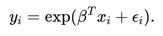
In certain cases, we might transform the target variable (e.g., taking a log transform of

y

). How does that transformation affect the assumption of normal error distribution and the interpretation of parameters?

If you model

under the assumption

it means that

is log-normally distributed, and

This can stabilize variance if the original

was skewed and the spread of the data grows exponentially with the mean. The MLE for

β

in the log-space is then the solution to minimizing the sum of squared residuals in log-space. The parameter interpretation changes:

• Coefficients become elasticities or percent changes in

  y

  for a one-unit change in the predictor, rather than absolute changes.

• Predictions in the original scale require exponentiation:

  

A subtlety is the “retransformation bias”: simply taking

exp⁡(predicted log value)exp(predicted log value)

can underestimate the true mean of

y

because

A common correction factor is

if you assume normality of residuals in log-space. Omitting it can bias your final predictions for

y.

When might we prefer a non-parametric or semi-parametric approach over a purely parametric Gaussian-based linear regression?

In some real-world problems, the functional relationship between features and target is not well-captured by a simple linear function (even after transformations). Additionally, strict distributional assumptions, such as Gaussianity for errors, may be incorrect. Non-parametric or semi-parametric approaches (e.g., kernel regression, spline-based regression, GAMs) can:

1. Capture more flexible relationships between predictors and the response.

2. Avoid heavy assumptions about parametric forms or exact normality of error distributions.

Potential downsides include:

• Higher risk of overfitting if the method is too flexible, especially in small samples.

• Computational complexity can be higher than classical linear regression methods, especially for large datasets.

• Interpretation of the resulting fit may be more complicated than a simple linear combination of features.

Edge cases occur if the data actually is linear but you apply an extremely flexible non-parametric model; you risk unnecessary complexity, slow training times, and potential for large variance in the estimates. Cross-validation to tune complexity is often critical.

How do we incorporate domain knowledge or constraints (e.g., positivity constraints on parameters) into maximum likelihood estimation for linear regression?

Sometimes, prior knowledge indicates that certain parameters should be non-negative or lie within a particular range (e.g., a growth rate parameter that cannot be negative). Standard OLS or unconstrained MLE might produce estimates violating these constraints. Approaches include:

1. Constrained Optimization: Solve the least squares problem under inequality constraints, for example using quadratic programming or a projected gradient method. This ensures the solution respects parameter bounds.

2. Reparameterization: Impose positivity by modeling a coefficient as

   

   , transforming an unconstrained parameter

   

   into a constrained space. Then MLE in terms of

   

   automatically enforces positivity in

   

3. Bayesian Approach with Informative Priors: Place priors that reflect domain knowledge, such as a half-Gaussian or half-Cauchy prior for non-negative parameters.

A subtlety is that imposing such constraints changes the geometry of the solution space, potentially complicating optimization. If the domain constraint is correct, the resulting estimates will be more physically or scientifically meaningful. If the constraint is incorrect or too restrictive, bias can be introduced.

If the true model is polynomial or has interaction terms, but we only fit a main-effects linear regression, does maximum likelihood under the Gaussian assumption still “work”?

Maximum likelihood estimation under a misspecified model (i.e., the model form

is not the true underlying function) is no longer guaranteed to produce unbiased estimates of the true relationship. Instead, it finds the best linear approximation in the sense of minimizing sum-of-squares under that linear constraint. While this might still yield a useful linear approximation, it does not capture the underlying non-linear or interaction structure if such terms are indeed significant.

In practice, to check for potential polynomial or interaction effects, researchers often:

• Conduct residual diagnostics to see if residuals systematically vary with certain predictors.

• Fit extended models with polynomial or interaction terms and compare model fit using criteria such as AIC/BIC or cross-validation error.

Pitfalls:

• Overfitting can occur if we blindly add higher-order terms or many interactions without verifying necessity.

• Interactions can introduce multicollinearity, so interpretability and variance of estimates might suffer.

What if the covariance of the noise is not diagonal but has a certain pattern (e.g., an AR(1) structure in time series), and how does maximum likelihood under that structure relate to least squares?

When residuals have serial correlation (like in time-series analysis with an AR(1) structure, meaning

depends on

), the naive OLS approach is no longer the maximum likelihood solution under the correct correlated error structure. The generalized least squares approach modifies the objective to account for the covariance structure

Σ

Maximizing the Gaussian log-likelihood with correlated errors is mathematically equivalent to minimizing the above generalized least squares objective. However, one must estimate or know

Σ

, often requiring iterative procedures (like Cochrane-Orcutt or more general maximum likelihood techniques).

A major pitfall is incorrectly specifying the correlation pattern. If the assumed covariance structure is far from reality, the estimates may be inconsistent or the confidence intervals inaccurate. On the other hand, if done correctly, modeling correlation can yield more efficient (i.e., lower-variance) parameter estimates and valid inference.