ML Interview Q Series: Logistic Regression Coefficients via Maximum Likelihood Estimation.

📚 Browse the full ML Interview series here.

How does a logistic regression model know what the coefficients are ?

Logistic regression determines its coefficients through the principle of maximum likelihood estimation. The model assumes a functional form that relates input features to the log-odds of a binary outcome. These coefficients are found by fitting the model to data, typically via an iterative optimization method such as gradient descent or a variant like L-BFGS.

Below is a detailed discussion of how logistic regression arrives at its coefficients

Logistic Regression Model Setup

In a binary classification setting, the logistic regression model predicts the probability of a positive class. It does so by modeling the log-odds (also called the logit function) of the probability as a linear function of the input features.

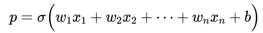
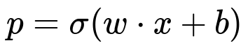
If x is the vector of input features, w is the vector of coefficients (weights), and b is the intercept (also called bias in some contexts), the model outputs:

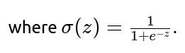
where p=P(positive class∣x) is the predicted probability of the positive class. The model thus connects the linear combination of inputs to probabilities via the logistic (sigmoid) function:

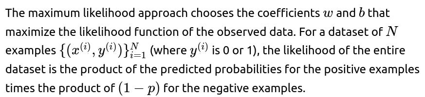
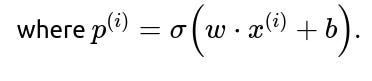
Finding the Coefficients Through Maximum Likelihood

To turn this into a more convenient summation, we often work with the log-likelihood:

Logistic regression solves the following optimization problem:

maximize ℓ(w,b)

or equivalently

minimize the negative log-likelihood −ℓ(w,b).

Training Through Gradient-Based Optimization

To find the coefficients that maximize the log-likelihood, many software packages use gradient-based approaches. By taking the gradient of the negative log-likelihood with respect to each coefficient and setting it to zero (or iteratively adjusting coefficients in the direction that reduces the loss), the algorithm converges to a coefficient vector w and intercept b that fit the data best under the logistic model assumptions.

In practice, libraries like scikit-learn (in Python) or other frameworks might use numerical optimization solvers (e.g., L-BFGS) or stochastic gradient descent. This process is iterative, adjusting w and b until convergence criteria (like a small change in the cost function between iterations or a maximum iteration count) are met.

Interpretation of the Coefficients

Practical Example in Python

Below is an example of fitting a logistic regression model in Python using scikit-learn and examining the learned coefficients:

import numpy as np
from sklearn.linear_model import LogisticRegression

# Example synthetic dataset
X = np.array([
    [0.2, 1.1],
    [0.4, 2.2],
    [0.8, 2.8],
    [1.0, 3.5],
    [1.5, 3.0],
    [2.0, 4.1]
])
y = np.array([0, 0, 0, 1, 1, 1])  # binary labels

# Fit logistic regression
model = LogisticRegression()
model.fit(X, y)

# Coefficients and intercept
coefficients = model.coef_
intercept = model.intercept_

print("Coefficients:", coefficients)
print("Intercept:", intercept)

In this code:

• 

• model.intercept_ gives the intercept b.

  

  Connecting Coefficients to Probabilities

It is common to transform the logistic regression output back into probability space. For a single input x, the predicted probability p is:

How Regularization Affects Coefficients

In many practical implementations (e.g., scikit-learn’s LogisticRegression with default settings), a penalty term (like L2 norm) is added to the cost function. This technique, known as regularization, shrinks the coefficient values toward zero to prevent overfitting. The presence of regularization means that the final learned coefficients strike a balance between fitting the training data and remaining small in magnitude, which promotes generalization.

Interpretation Nuances and Feature Scaling

Subtle Points About Odds vs. Probability

Summary of Key Observations

Logistic regression finds its coefficients by maximizing the likelihood of the observed data. Those coefficients have a direct linear relationship with the log-odds of the positive class. A positive coefficient implies that increasing that feature’s value increases the log-odds (and typically the probability) of the event. A negative coefficient implies the opposite. Regularization and feature scaling can alter coefficient magnitudes and thus influence how easily you can interpret them numerically.

How might you explain coefficient interpretation in simpler terms?

What if the dataset is unbalanced? How does that affect the coefficients?

Class imbalance can influence the magnitude of coefficients because the model attempts to separate the positive class from the negative class efficiently. In an imbalanced dataset, the model might learn that predicting the majority class is safer, potentially shrinking certain coefficients or biasing the intercept. Techniques like class weighting, oversampling of the minority class, or undersampling of the majority class can help achieve more balanced coefficient learning. The mathematical process (maximum likelihood estimation) remains the same, but the model sees a different relative penalty for misclassifying minority-class examples when class weights are used.

Why do some software packages fit logistic regression using gradient descent vs. advanced solvers like L-BFGS?

Both gradient descent and advanced solvers like L-BFGS or Newton’s method rely on gradients of the cost function. However, advanced solvers often converge faster on small to medium-sized datasets and automatically adapt step sizes or approximate second-order information. Pure stochastic gradient descent can be more suitable for very large datasets where computing exact gradients at every iteration is expensive. Either way, the learned coefficients are solutions to the same underlying optimization problem, just arrived at via different numerical methods.

How do we diagnose coefficient stability?

If coefficients drastically change when:

• Slightly altering the training data

• Dropping or adding a feature

• Modifying regularization strength

this can indicate instability or high correlation between features. Highly correlated predictors (multicollinearity) can cause the model to distribute weights in an unstable manner. Checking variance inflation factors (VIF) or using dimensionality reduction techniques might help. The stability of coefficients is essential for interpretability; in an unstable scenario, small changes in data can lead to large changes in coefficient values, making it difficult to rely on their interpretation.

When is logistic regression not appropriate?

Logistic regression can be insufficient if the data exhibit a highly complex decision boundary that cannot be well-approximated by a linear log-odds function. In such cases, more flexible models (e.g., random forests, gradient-boosted trees, neural networks) might better capture patterns. Additionally, logistic regression assumes a relationship between features and the log-odds that is linear. If strong interactions or nonlinear effects are present but not included in the model (e.g., polynomial or interaction terms), the logistic regression fit can be poor. Still, logistic regression remains popular for its simplicity, interpretability, and efficiency, especially with high-dimensional but well-structured data.

How do we handle continuous vs. categorical variables in logistic regression?

Continuous variables can be included directly after optional scaling. Categorical variables often require encoding. Typically, one uses one-hot encoding or dummy variables. Each category, except one reference category, gets its own indicator feature. The coefficient associated with that indicator represents the effect of being in that category relative to the reference category on the log-odds scale. If there are many categories or high-cardinality features, one may need regularization or dimensionality reduction to avoid overfitting and coefficient instability.

Why is coefficient interpretation trickier for logistic regression than linear regression?

In linear regression, a one-unit increase in a feature corresponds to a direct increase or decrease in the predicted outcome by the coefficient’s magnitude. In logistic regression, the coefficient directly affects the log-odds rather than the probability. Because probability is bounded between 0 and 1, the change in probability for a one-unit change in a feature depends on the current value of all features passed through the sigmoid. Thus, a coefficient has a more straightforward linear meaning only in log-odds space, and not in direct probability space.

Could the sign of a coefficient ever be misleading?

The sign of the coefficient should always reflect whether that feature increases or decreases log-odds. However, if there is a strong correlation among features, the model might assign a negative sign to one correlated feature and a positive sign to another to partially cancel out. This scenario can create confusion in interpretation, so domain knowledge is essential. Also, sign flips can occur if a feature correlates with omitted confounding variables. Checking partial dependence or performing a more thorough analysis of interactions can clarify these subtleties.

How do we decide whether a coefficient is important in logistic regression?

One approach is to look at the magnitude of the coefficient in log-odds space or examine its exponentiated value to see how it scales the odds. Another approach is to assess the statistical significance via a Wald test or by inspecting confidence intervals around coefficients. Alternatively, in a purely predictive context, a feature’s importance might be evaluated by measuring the drop in model performance when that feature is removed. Each method offers a different perspective on importance—some are more interpretability-focused, while others are more predictive-performance-focused.

What if the model does not converge?

If the algorithm fails to converge (e.g., the solver hits a maximum iteration limit), possibilities include:

• Very high multicollinearity

• Extremely large feature values

• Very strong regularization parameter (or very small regularization strength leading to near-infinite coefficients)

• Poor choice of learning rate when using gradient-based methods

Addressing these might involve standardizing or normalizing features, removing highly correlated variables, or tuning regularization parameters. Convergence issues in logistic regression typically manifest as the solver or gradient descent not settling to stable coefficient values.

How would you handle interpretability if you scale your data?

Could you provide a quick code example illustrating the coefficient interpretation in odds?

import numpy as np
from sklearn.linear_model import LogisticRegression

X = np.array([
    [1.0],
    [2.0],
    [3.0],
    [4.0]
])
y = np.array([0, 0, 1, 1])

model = LogisticRegression(fit_intercept=True)
model.fit(X, y)

coef = model.coef_[0][0]
intercept = model.intercept_[0]

odds_multiplier = np.exp(coef)

print("Coefficient (log-odds):", coef)
print("Odds multiplier:", odds_multiplier)
print("Intercept:", intercept)

In this single-feature case, coef is w, and odds_multiplier = exp(w). If, for example, coef is around 0.69, odds_multiplier would be around 2.0, indicating that for every one-unit increase in the feature, the odds double (assuming other features are held constant, though here we have only one feature).

In summary, how does a logistic regression model know its coefficients?

It finds the coefficients by maximizing the likelihood of the observed binary outcomes under the assumed logistic model. The iterative optimization method (gradient descent, L-BFGS, or similar) systematically updates the coefficients until it converges on values that best separate the classes according to the logistic function. Those resulting coefficients reflect how each input feature influences the log-odds of the predicted probability.