ML Interview Q Series: Logistic Regression: Maximizing Log-Likelihood for Binary Classification Modeling.

📚 Browse the full ML Interview series here.

40. Describe the model formulation behind logistic regression (two-class case). How do you maximize the log-likelihood of a given model?

This problem was asked by Stripe (Hard).

The logistic (sigmoid) function is

which ensures that the output is between 0 and 1 for any real number z. Thus, for each input x, the model’s predicted probability of the label y=1 is

Correspondingly,

The summation is taken over all training samples. Maximizing this L(w) is equivalent to minimizing the negative log-likelihood, which is often referred to as the cross-entropy loss. In practice, we typically apply a numerical optimization method such as gradient ascent (to directly maximize L(w)) or gradient descent (to minimize the negative of L(w)). For convenience in many libraries, it is coded as minimizing the negative log-likelihood.

Summing over the entire dataset, the gradient becomes

By iteratively updating the parameters in the direction of the gradient (or in the opposite direction of the negative gradient, depending on which sign convention one chooses for the step size), the model converges to parameters that locally maximize the log-likelihood. In practice, one often uses variants of gradient descent (like stochastic or mini-batch gradient descent) for computational efficiency on larger datasets.

Implementation in Python (illustration of gradient descent)

import numpy as np

def sigmoid(z):
    return 1.0 / (1.0 + np.exp(-z))

def compute_loss_and_gradients(X, y, w):
    # X is of shape (N, d), y is of shape (N,), w is of shape (d,)
    # N: number of samples, d: number of features
    N = X.shape[0]
    predictions = sigmoid(X.dot(w))  # shape (N,)
    # Negative log-likelihood (we typically minimize this)
    loss = - np.mean(y * np.log(predictions + 1e-15) +
                     (1 - y) * np.log(1 - predictions + 1e-15))
    # Gradient of the negative log-likelihood
    grad = (1.0 / N) * X.T.dot(predictions - y)  # shape (d,)
    return loss, grad

def fit_logistic_regression(X, y, lr=0.01, epochs=1000):
    # Initialize parameters
    w = np.zeros(X.shape[1])
    for epoch in range(epochs):
        loss, grad = compute_loss_and_gradients(X, y, w)
        # Gradient descent: move w in the opposite direction of the gradient
        w -= lr * grad
    return w

# Example usage:
# Suppose X_train is shape (N, d), y_train is shape (N,)
# w_opt = fit_logistic_regression(X_train, y_train, lr=0.1, epochs=2000)
# Then for inference, you can compute preds = sigmoid(X_test.dot(w_opt)) > 0.5

Below are several follow-up questions that might arise in an interview, each answered in a detailed way to highlight the deeper understanding of logistic regression.

40-a. Why do we use the logistic (sigmoid) function in logistic regression instead of just applying a linear model directly to classify?

40-b. Why is logistic regression considered a linear model when the hypothesis has a sigmoid function?

40-c. How do you handle the maximization of the log-likelihood in practice, and why don’t we have a closed-form solution for logistic regression like we do in linear regression?

40-d. Can you derive the gradient of the log-likelihood function for logistic regression?

Summing over all N samples gives

In practice, we typically compute this gradient over mini-batches or over the entire dataset in each iteration of gradient-based optimization.

40-e. What is the connection between maximum likelihood in logistic regression and cross-entropy loss minimization?

Maximizing the log-likelihood

is equivalent to minimizing the negative log-likelihood:

40-f. In logistic regression, are there ways to deal with class imbalance?

Yes. Class imbalance occurs when one class is much more frequent than the other. Several approaches exist: One approach is to introduce class weights in the log-likelihood function so that misclassifying the minority class is penalized more heavily. This effectively re-scales the gradient contributions for examples of the minority class. Another approach is to perform oversampling of the minority class or undersampling of the majority class. Additionally, advanced methods include synthetic sample generation techniques such as SMOTE (Synthetic Minority Over-sampling Technique). Regardless of the specific method, the core logistic regression model remains the same, but the training procedure or data sampling strategy is adjusted to compensate for the imbalance.

40-g. What is Newton’s method in logistic regression, and how does it relate to iteratively reweighted least squares?

Newton’s method is a second-order optimization approach for finding maxima or minima of a function. In logistic regression, it can be used to find the maximum of the log-likelihood by incorporating the Hessian matrix (matrix of second derivatives) in the parameter update. Specifically, if g is the gradient and H is the Hessian, a Newton update for maximizing the log-likelihood is

For logistic regression, the resulting form of the Hessian leads to what is known as iteratively reweighted least squares (IRLS). Essentially, each iteration of Newton’s method solves a weighted least squares problem. Although Newton’s method typically converges in fewer iterations than first-order methods, it can be more computationally expensive on high-dimensional problems because it requires calculating and inverting the Hessian. Libraries like scikit-learn and others often implement logistic regression training via second-order methods for smaller or medium scale datasets, but for very large datasets, stochastic gradient descent or its variants might be more efficient.

40-h. What are the limitations of logistic regression compared to more flexible models?

Logistic regression is fundamentally a linear model in terms of the input space, so it cannot naturally capture non-linear decision boundaries unless you manually engineer non-linear transformations of features or use kernels. It also assumes data features combine additively on the log-odds scale, which might not hold in all real-world problems. Furthermore, when classes are not linearly separable in the given feature space, logistic regression has limited representational power unless feature engineering or polynomial expansions are introduced. More flexible models like random forests, gradient boosting machines, or neural networks can capture more complex decision surfaces but may require more data and more careful hyperparameter tuning.

40-i. How do you interpret the coefficients of logistic regression?

40-j. How do you address overfitting in logistic regression?

40-k. Why is the log-likelihood function in logistic regression concave in terms of parameters (making the negative log-likelihood convex) and why does that matter?

40-l. In practice, how do you initialize parameters in logistic regression, and does initialization matter?

A common default is to initialize the weight vector w to zeros, or small random values drawn from some distribution. In logistic regression, if you do not have regularization that breaks symmetry or if you do not have strongly correlated features, the zero initialization is typically a decent starting point because logistic regression’s loss landscape is generally well-behaved (convex in the negative log-likelihood sense). In large-scale or complex feature spaces, random initialization can sometimes help break degeneracies. However, for convex problems like logistic regression, the algorithm will converge to the same global optimum regardless of the starting point (barring floating-point issues or certain forms of regularization).

40-m. Could logistic regression work with non-linear feature transformations?

Yes. To capture non-linear relationships, one can transform the input features before feeding them into logistic regression. For instance, you can add polynomial features or apply custom transformations (e.g., sin⁡(x), exp⁡(x), etc.). The logistic regression model then becomes linear in the transformed feature space, even though that transformation may capture non-linear effects in the original input space. This is one way to enhance the representational power of logistic regression without moving to more complex models. However, feature engineering may require domain expertise and can still be limited compared to truly non-linear models like neural networks or tree-based ensembles that automatically learn such non-linearities.

40-n. What if the classes are perfectly separable by a hyperplane in logistic regression?

When the data is linearly separable, the maximum-likelihood solution in logistic regression can send the magnitude of w to infinity. This happens because you can keep pushing the decision boundary to classify all points perfectly with increasing confidence, leading to extremely large weights in the direction that separates the classes. In practice, this causes unstable parameter growth. Regularization (e.g., L2 or L1) forces the parameters to remain finite by penalizing large values. This is a key reason to include some form of regularization in logistic regression, especially in high-dimensional settings where perfect separation might be more easily achieved.

40-o. Do outliers affect logistic regression, and how does that compare to linear regression?

Logistic regression is somewhat more robust to extreme outliers in the feature space than linear regression because it essentially cares about the decision boundary in classification tasks rather than predicting a continuous target value. An extreme outlier can pull the decision boundary somewhat, but if the outlier belongs to a certain class, the logistic model is limited in how drastically that single point can shift the boundary, as long as the majority distribution remains consistent. That said, outliers in the input space that are mislabeled or extremely unusual can still affect logistic regression. Techniques such as robust scaling, outlier removal, or re-weighting strategies might still be employed if outliers pose a problem.

40-p. In high-dimensional settings, does logistic regression suffer from the curse of dimensionality?

Yes. When the number of features is very large relative to the number of observations, logistic regression can overfit, and the variance of parameter estimates increases. Regularization is essential in this scenario. L1 regularization (lasso) can help in performing feature selection by driving some coefficients to zero, effectively discarding redundant or less important features. L2 regularization helps by shrinking coefficients but does not automatically drive them to zero. Either way, with sufficiently strong regularization and possibly dimensionality reduction (e.g., PCA) or feature selection, logistic regression can still be effective in high-dimensional problems.

40-q. How does one apply logistic regression in an online learning scenario?

Online learning for logistic regression typically uses stochastic gradient descent (SGD). Each incoming data point (or small batch) is used to update the weights:

1. Compute the predicted probability for the new sample using the current weights.

2. Compute the gradient of the log-likelihood for that single sample (or small batch).

3. Update the weights in the direction that maximizes the log-likelihood (or equivalently, reduces the negative log-likelihood).

With a properly chosen learning rate schedule and possible use of regularization, the model parameters can adapt incrementally as new data arrives, making logistic regression suitable for large-scale or streaming data problems.

---

Below are additional follow-up questions

How do we handle probability calibration in logistic regression when the predicted probabilities seem poorly aligned with real-world frequencies?

One subtle challenge in real-world applications of logistic regression is ensuring that the model’s predicted probabilities align closely with empirical frequencies of the positive class. For instance, if your model outputs a probability of 0.7 for 100 instances, ideally you would want around 70 of those instances to be truly labeled “positive.” However, sometimes logistic regression (or any probabilistic classifier) might be miscalibrated—meaning the predicted probabilities do not reflect true likelihoods.

To handle miscalibration, you can:

• Perform calibration on top of the raw probabilities. Common methods include Platt scaling or isotonic regression. In Platt scaling, you fit a secondary logistic function to map the original scores or probabilities to better-calibrated probabilities. Isotonic regression is a non-parametric approach that fits a piecewise constant non-decreasing function to align predicted probabilities with observed frequencies.

• Adjust decision thresholds if your goal is classification. If the main objective is not the raw probability but rather a classification outcome (like deciding if something is spam or not), you could tune the threshold beyond the default 0.5 to improve metrics such as F1-score, precision, recall, or a cost-sensitive measure. However, tuning the threshold alone usually does not fix probability miscalibration; it just improves classification metrics.

• Gather more representative data. If the training dataset distribution differs significantly from the real-world distribution, calibration can drift. Ensuring the training set is representative helps align probabilities to real event frequencies.

A subtle pitfall is that even though logistic regression theoretically can produce well-calibrated probabilities (under correct model specification and enough data), in practice it might still exhibit calibration errors due to regularization (especially strong regularization that shrinks coefficients excessively), data shift, or certain class imbalance situations.

How can logistic regression be extended for multi-class classification beyond the two-class case?

Although the original logistic regression formulation focuses on binary classification, there are two main strategies for multi-class problems:

• One-vs-Rest (OvR, also known as One-vs-All). You train one binary logistic regression classifier per class, where that class’s samples are considered “positive” and all other classes’ samples are considered “negative.” For prediction, you typically pick the class whose classifier returns the highest predicted probability (or the largest logit). A potential edge case arises if multiple classifiers predict similar probabilities, leading to ties or near-ties. Handling these cases might require tie-breaking rules or confidence intervals around the probabilities.

• Softmax (multinomial) logistic regression. Instead of modeling the probability of a single class via a sigmoid function, you use the softmax function over linear logits:

How do you check for convergence in logistic regression and decide when to stop the iterative optimization?

During training, especially with gradient-based or quasi-Newton optimization, you can monitor:

• The magnitude of the gradient. When the gradient’s norm falls below a certain threshold, it often indicates that the parameters are near an optimum.

• A maximum iteration or time budget. In large-scale scenarios, it might be impractical to wait for an extremely tight convergence. You often use early stopping after a certain number of iterations or once a validation metric shows minimal improvement.

A subtle edge case is “ill-conditioned” problems: if some features are nearly linearly dependent or the data is extremely sparse, the Hessian (in second-order methods) might be close to singular, making convergence checks tricky. In such cases, adding or increasing regularization helps.

Why might we consider ordinal logistic regression instead of standard logistic regression when classes have an inherent order?

In some classification tasks, labels have a natural ordering (e.g., “negative,” “neutral,” “positive” in sentiment analysis, or “low,” “medium,” “high” in quality scores). Standard logistic regression treats these classes as unordered categories if done in a one-vs-rest or multinomial framework. Ordinal logistic regression, by contrast, exploits the fact that the classes have a rank. This is usually accomplished by assuming different intercepts (thresholds) for each ordered category, with a single shared set of coefficients governing the effect of features.

Using ordinal logistic regression:

• Better captures scenarios where misclassifying a “low” label as “high” is fundamentally worse or has a different cost than misclassifying it as “medium.” The ordinal approach recognizes that “low < medium < high.”

• Often yields more interpretable models in situations where you want to see how an increase in a feature affects the probability of being in a higher-ordered category versus a lower one.

However, potential pitfalls include:

• Model complexity. While the coefficient vector is shared across thresholds, fitting multiple thresholds can still lead to challenges if the data is limited in certain categories.

• Violations of the proportional odds assumption. Ordinal logistic regression often assumes the effect of each feature is constant across different thresholds. If that assumption doesn’t hold, the model can be biased.

How is logistic regression related to the exponential family of distributions?

Logistic regression is a member of the generalized linear models (GLMs). Specifically, the Bernoulli distribution for binary outcomes is an exponential-family distribution with:

When would we choose a probit model over logistic regression, and what are the differences?

Probit regression is another way to model binary outcomes. Instead of the logistic function, it uses the cumulative distribution function (CDF) of the standard normal distribution (the “probit” function). The difference between probit and logistic lies in the shape of these link functions: the probit CDF is a bit steeper in the tails than the logistic function. In practice, they often yield very similar performance and predictions.

Reasons you might pick a probit model include:

• Historical or domain-specific convention, especially in certain fields such as econometrics, psychometrics, or certain medical applications.

• The probit link aligns with latent-variable interpretations, for example, if you believe there’s an underlying normally distributed propensity that triggers a 0 or 1 outcome at some threshold.

Pitfalls include the fact that the probit model does not have a closed-form for the negative log-likelihood gradient (it involves the pdf of the normal distribution), so computations can be slightly more expensive. Also, interpretability of coefficients in probit is almost identical to logistic in spirit (still a linear effect on a latent scale), but log-odds interpretation is not as direct as in the logistic case.

How can correlated features or multicollinearity affect logistic regression estimates?

When features are highly correlated (multicollinearity), logistic regression’s parameter estimates can become unstable or very large in magnitude. The model might struggle to distinguish which feature is truly driving the prediction because they supply nearly redundant information. Some symptoms or pitfalls:

• Large variance in coefficient estimates. Slight changes in the training data can cause large swings in parameter values.

• Overfitting. If two or more features almost duplicate each other, the model may latch onto spurious signals unless adequately regularized.

• Numerical instability in iterative methods. The Hessian matrix can become nearly singular, slowing convergence or causing large parameter updates.

Countermeasures include:

• Feature selection or dimensionality reduction (like PCA) to remove near-duplicate features.

• Stronger regularization (L2 in particular helps “spread out” the importance across correlated features, while L1 might zero out some correlated features completely).

• Domain-informed grouping or transformation of correlated features. For example, if you have separate but highly correlated measurements of the same underlying quantity, you might average them or pick the single best measure.

What does it mean to compute confidence intervals or p-values for the coefficients in logistic regression?

Because logistic regression is a parametric method with coefficients interpreted on the log-odds scale, classical statistics often seeks to estimate the uncertainty of these coefficients. Confidence intervals or p-values can be derived from the approximate covariance matrix of the parameter estimates, which typically comes from inverting the observed (or expected) Fisher information (i.e., the Hessian of the negative log-likelihood).

Steps to obtain them:

Pitfalls arise when:

• Data is sparse or perfectly (or near perfectly) separable. In this case, the Hessian can be degenerate, making confidence intervals infinite or highly unreliable.

• Regularization is in effect. Standard formulae for confidence intervals do not directly account for the penalization. Tools like bootstrapping or Bayesian treatments might be more appropriate if heavy regularization is used.

How does kernel logistic regression work, and when is it used?

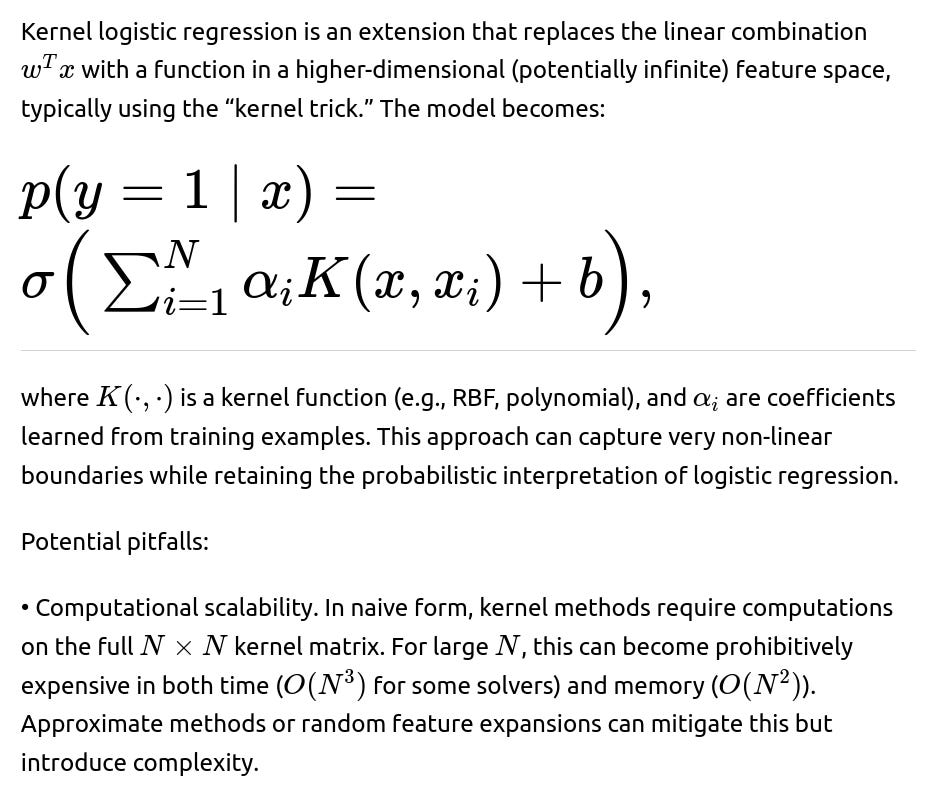
• Hyperparameter tuning. Choosing the right kernel and kernel hyperparameters (like the RBF width) can be tricky. Overly flexible kernels can lead to overfitting without careful regularization or cross-validation.

How do we handle “near-zero or near-one” predictions in code, and why is it important?

The typical solution is to clip the predicted probabilities away from exact 0 or 1:

eps = 1e-15
pred_clipped = np.clip(predictions, eps, 1 - eps)
loss = - np.mean(y * np.log(pred_clipped) +
                 (1 - y) * np.log(1 - pred_clipped))

Pitfalls if you do not clip:

• NaN or inf values that break the training loop. • Inconsistent gradient updates, causing the optimizer to fail to converge.

In real-world scenarios, you might find that strong signals or heavily imbalanced data produce extremely confident predictions (e.g., 0.999999999). While the logistic model is suggesting near-certain classification, from a numerical perspective it is safer to clip or add small smoothing constants to maintain stable computation.

How do you adapt logistic regression to extremely large datasets with billions of samples?

When data is extremely large:

• Batch gradient descent over the entire dataset each iteration might be infeasible. Instead, you use stochastic gradient descent (SGD) or mini-batch gradient descent, processing chunks of data at a time. This reduces memory usage and can speed up convergence in practice.

• Regularization and early stopping become more important because large datasets might contain noisy or redundant features.

• Parallelization or distributed computing frameworks (Spark, Hadoop, parameter servers) can be used. For instance, you can distribute the computation of gradient partial sums across multiple workers, then aggregate them to update the parameters.

• Specialized solvers like asynchronous SGD or Hogwild! can exploit multi-threading or multi-processor architectures. However, concurrency can introduce updates that are not strictly sequential, risking “race conditions” in parameter updates. Empirically, these methods can still converge quickly for logistic regression because the objective is relatively well-behaved.

One subtle challenge is deciding how to shuffle or sample the data. If you have 1 billion samples, ensuring that you are not missing entire sub-populations in any training epoch is crucial. Data sampling or partitioning strategies significantly impact model performance. Also, re-initializing or re-shuffling the data each epoch might be computationally costly. Practical solutions sometimes fix an ordering for streaming data but ensure enough diversity in each mini-batch.

What if some of the labels in the dataset are noisy or even adversarial? Can logistic regression still learn effectively?

Logistic regression can be somewhat robust to label noise if the fraction of noise is not too high, but it remains sensitive to systematic or adversarial mislabeling. Since the log-likelihood is maximized under the assumption that labels are correct given the model’s probabilities, systematically incorrect labels can bias the parameter estimates.

Strategies include:

• Outlier or mislabeled instance detection. You can look for samples whose features are extremely atypical for their labeled class or whose predicted probability from a partial model is near 0 or 1 but with the opposite label. These might be re-examined or removed.

• Robust loss functions. A typical cross-entropy can amplify the effect of mislabeled samples that produce large negative log-probabilities. Some robust statistics approaches propose alternative link or loss functions, but these are less standard than for linear regression.

• Active learning or data verification. Instead of passively taking the entire dataset at face value, carefully recheck suspicious data points (manual or automated auditing). This is especially vital if there is a risk of adversarial labeling, such as spam detection systems.

A key pitfall is that logistic regression does not have any intrinsic mechanism to guess that a label might be incorrect. Unlike some robust estimators, classical logistic regression simply trusts the data. Heavy label noise can degrade performance significantly, so data quality checks remain critical.

Can logistic regression output be interpreted in a Bayesian way to get posterior distributions on parameters?

Yes. You can place priors on w (e.g., a Gaussian prior for each coefficient) and then update these priors with data likelihood according to Bayes’ rule. The resulting posterior distribution over w is typically not analytically tractable, but approximate inference methods (e.g., Laplace approximation, variational inference, Markov Chain Monte Carlo) can be used. This approach yields a Bayesian logistic regression model, which provides:

• Posterior distributions over coefficients, allowing more nuanced uncertainty estimates than a single point estimate.

• Automatic regularization. A Gaussian prior on w is analogous to L2 regularization but framed probabilistically.

Pitfalls or complexities include:

• Computation can be more involved, especially with MCMC for larger datasets. • The approximate posteriors might be sensitive to hyperparameter choices in the prior (e.g., the variance of the Gaussian). • With extremely large data, approximate methods need to be scaled carefully, or you might revert to simpler MAP estimates that reduce to classical regularized logistic regression.

How might you interpret the bias/intercept term in logistic regression separately from the coefficients?

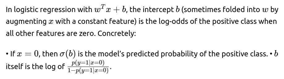
Potential real-world pitfalls:

• If your features are not mean-centered or zero is not a meaningful reference point (e.g., an age feature where zero is not in the domain of interest), then interpreting b can be nonsensical or less intuitive. • In practice, the intercept simply shifts the decision boundary up or down in log-odds space. It ensures that the proportion of positive predictions (on average) aligns well with the training data if the rest of the coefficients do not systematically correct for it.

How do we handle extremely unbalanced features, such as one feature having extremely large values compared to others?

Feature scaling is often important for stable training:

• If one feature is on a vastly larger numeric scale, gradient steps involving that feature might dominate, causing instability or slow convergence. • Normalizing or standardizing features (e.g., subtract mean, divide by standard deviation) can help gradient-based methods converge more smoothly. • Even if your final interpretability requires the original scale, you can still keep track of transformations and invert them post-training for interpretability. • Another approach is automated regularization or adaptive methods (like AdaGrad, RMSProp, Adam in neural network contexts). For plain logistic regression without advanced optimizers, a big difference in scale can still hamper standard gradient descent or Newton’s method.

A subtlety is that if certain features must remain in their raw scale (e.g., if zero has real significance), consider partial transformations or carefully controlling step sizes. You do not necessarily want to lose meaningful interpretability in domain-specific tasks.

Could logistic regression be combined with feature embeddings, for instance, in NLP tasks or categorical variable encodings?

Yes, logistic regression can incorporate embeddings for categorical or text features. For example:

• In an NLP scenario, each word or document might be represented by a pre-trained embedding (e.g., from word2vec or GloVe). Then logistic regression uses these embedding vectors as input features. • In dealing with large numbers of categories in structured data (like hundreds of thousands of product IDs), you can learn low-dimensional embeddings for these categories separately, then feed those embeddings into logistic regression.

The logistic regression portion remains linear on the embedding dimension. The embedding process itself can be pre-trained or even jointly learned in some specialized frameworks. Pitfalls:

• Overfitting can occur if the embedding dimension is large and the training set is not sufficiently large. • The learned embeddings might not capture context as well as deep neural networks that fine-tune embeddings end-to-end with a more flexible architecture. • If embeddings are static (pre-trained and frozen), the logistic regression will only be as good as the pretrained representation’s alignment with your specific task.

Still, this approach is appealing in certain large-scale industrial tasks (e.g., advertising or ranking) where logistic regression is valued for interpretability and speed, but you still want to capture some notion of semantic or categorical similarity via embeddings.

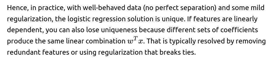
Is the negative log-likelihood in logistic regression guaranteed to be strictly convex, and how does that affect uniqueness of solutions?

• Perfect separation or near-separation can lead to directions in parameter space that continue to improve the likelihood without bound, pushing w to extremely large magnitude. In these cases, the solution is not unique in an unconstrained sense (it diverges).

• If you introduce strict convexity via regularization (e.g., an L2 term), then the regularized objective becomes strictly convex, guaranteeing a unique global minimum even in near-separable scenarios.

How can threshold tuning or cost-sensitive adjustments be incorporated into logistic regression?

By default, logistic regression uses a threshold of 0.5 to decide between predicted classes 0 or 1. But for applications with asymmetric costs (e.g., false positives vs. false negatives have different business impacts), you can shift the threshold. For instance, if a missed detection is worse than a false alarm, you might reduce the threshold below 0.5. You can find the optimal threshold by:

• Plotting the ROC curve or Precision-Recall curve and selecting a threshold that maximizes a chosen metric (e.g., F1, precision at a certain recall, cost-based function).

• Using methods like a cost matrix specifying the penalty of each outcome (TP, FP, FN, TN) and searching for the threshold that minimizes overall expected cost on a validation set.

A subtle point is that changing the threshold does not alter the fitted parameters of logistic regression itself; it just changes how you convert predicted probabilities into discrete decisions. If the data distribution changes, you might need to recalibrate or retune the threshold. Another edge case arises if you have extremely unbalanced data with rare positives—sometimes the logistic regression might produce systematically low probabilities, and a threshold of 0.5 might yield very few positive predictions. Adjusting the threshold or combining class-weighting is then critical.

How might logistic regression interact with fairness constraints or bias in real-world datasets?

Logistic regression, like most supervised learning methods, can encode biases present in the training data. For instance, if certain protected groups are underrepresented or historically disadvantaged, the model might learn coefficients that systematically disadvantage those groups. Potential approaches to mitigate these issues include:

• Preprocessing: Remove or obfuscate sensitive features (e.g., race, gender) or apply re-weighting to create a more balanced effective dataset. But sensitive information can still be inferred indirectly from other correlated features.

• In-processing constraints: Modify the training objective to include fairness constraints or regularization terms that enforce demographic parity, equality of opportunity, or other fairness criteria. This is more complicated than standard logistic regression and typically involves custom optimization.

• Post-processing: Adjust the decision threshold per subgroup or apply calibration within each subgroup. This ensures consistent false positive/false negative rates across protected groups, but can sometimes reduce overall accuracy.

A critical pitfall is that removing explicit sensitive features does not necessarily remove bias. Data can contain proxies (e.g., zip code might correlate with race). Also, fairness is multi-faceted, and focusing on one fairness metric (like demographic parity) can harm another (like equal opportunity). In an industrial environment, deploying logistic regression in contexts like hiring or lending must carefully account for these constraints and legal considerations.

How do we systematically select hyperparameters like the regularization strength in logistic regression?

Logistic regression can be augmented with hyperparameters, such as:

• λ in L2-regularized logistic regression (or α in L1-regularized regression). • The penalty type (L1, L2, elastic net).

To select these hyperparameters, typically you:

• Use cross-validation, splitting the data into training and validation folds. • Train a series of models with different λ values and pick the one that performs best on a validation metric (could be accuracy, ROC AUC, F1, or log-loss). • Optionally do nested cross-validation or a separate hold-out test set to ensure robust performance estimation.

Pitfalls include:

• Overly large λ might overshrink coefficients, hurting predictive performance. • Overly small λ might allow overfitting, leading to large coefficient magnitudes. • L1 vs. L2 or a combination might be chosen based on domain needs (e.g., interpretability via feature selection vs. stable parameter estimates). • Overfitting the validation set by extensive hyperparameter search can occur; meta overfitting is mitigated by careful cross-validation.

How might logistic regression behave if we only have a tiny dataset?

In low-data regimes, logistic regression might suffer from high variance in parameter estimates, especially if the dimensionality of features is moderate or high. Each parameter’s estimate becomes quite uncertain, and if the classes are poorly represented, the model might easily misrepresent log-odds.

Strategies to cope:

• Stronger regularization: In a very data-scarce scenario, a high level of L2 regularization helps stabilize coefficients. Bayesian priors (e.g., a fairly tight Gaussian prior) can further regularize the solution.

• Feature reduction: Eliminating or combining features lowers dimensionality. This can drastically reduce variance in parameter estimates.

• Informative priors or domain knowledge: If you have prior knowledge about likely directions or magnitudes of coefficients, a Bayesian approach can incorporate that. Or you might fix certain coefficients if you are confident about them.

A subtlety is that logistic regression, being a relatively simple parametric model, can sometimes perform better than more complex models when data is extremely limited, precisely because it has fewer parameters to learn. But you must be cautious about interpretability claims in extremely small datasets because standard errors on coefficients can be large.

How would you diagnose issues in a trained logistic regression model?

Common diagnostic tools include:

• Residual analysis or deviance residuals. Plotting how each instance deviates from the model’s predicted probability can highlight systematic under- or over-prediction for certain feature ranges.

• Checking rank ordering. For binary classification tasks, see if predictions are ordered correctly relative to actual outcomes. If the model is systematically reversed in some sub-population, that indicates a mismatch.

• Confusion matrix or more advanced metrics (ROC curves, Precision-Recall). Evaluate if the model systematically confuses positives and negatives, or if certain subgroups are misclassified at higher rates.

• Coefficient sanity checks. Look at the sign and magnitude of coefficients—do they align with domain intuition? If a domain-expected positive relationship is showing as highly negative, that might reveal data quality problems or confounding variables.

• Checking for multi-collinearity. Variance Inflation Factor (VIF) can reveal if any feature is highly collinear with others, potentially destabilizing estimates.

Edge cases include:

• The model might look superficially fine on aggregate metrics, yet fail drastically on certain sub-populations. Disaggregated analysis (by region, demographic group, time period) can catch these failures. • Overfitted models might appear to have excellent training performance but fail once deployed if new data distribution differs from the training set. Monitoring performance over time post-deployment is crucial.

How does logistic regression relate to the Bayes decision rule if the likelihoods and priors are known?

In a Bayesian classification context, the optimal decision rule for two classes is to pick the class that maximizes the posterior probability p(y=1∣x). If we assume a linear model in the log-odds space plus a Bernoulli likelihood, logistic regression emerges naturally from maximizing the likelihood of training data under this model assumption. Equivalently, if we assume:

• Class priors p(y=1) and p(y=0). • A parametric form for the likelihood ratio or the log-likelihood ratio.

In short, logistic regression can be seen as a discriminative model implementing the Bayes decision rule under a specific parametric log-odds assumption. A pitfall is that if the true underlying process is more complex, the model is only an approximation, and ignoring that complexity can degrade performance.