
ML Interview Q Series: LSTM's Forget, Input, and Output Gates: Mastering Long-Term Dependencies.

📚 Browse the full ML Interview series here.
LSTM Gates: LSTMs were designed to address RNN limitations. Describe the purpose of the forget gate, input gate, and output gate in an LSTM cell. How do these gates work together to control the cell state and hidden state, allowing the network to maintain long-term information (and decide what to forget) over many time steps?
Understanding LSTM architectures is often the key to seeing how they can store and manipulate information over many time steps. Unlike standard RNNs, which can struggle with vanishing or exploding gradients when dealing with long sequences, LSTMs tackle these issues through an explicit internal state called the cell state, combined with three gates that regulate the flow of information.
The gates in an LSTM cell are the forget gate, the input gate, and the output gate. Each of these gates is typically implemented as a sigmoid function (ranging between 0 and 1), and each gate’s output is used to filter or scale different aspects of the information passing through the cell. By combining these three mechanisms, the LSTM can carry information forward for long durations, effectively alleviating many of the issues associated with training RNNs over long sequences.
Understanding the cell state itself is critical. The cell state is designed to be a vehicle for transferring information across many time steps. The gates collectively decide how to update this cell state at each step.
Role of the Forget Gate
The forget gate determines which parts of the existing cell state need to be retained and which parts should be removed. This is crucial for tasks where old information is no longer relevant, and it helps the LSTM focus on the information that still matters. The forget gate output multiplies the current cell state, thus “forgetting” certain components of the cell state. If the forget gate outputs values close to 1 for a component, it is kept; if it outputs something close to 0, that component is forgotten.


An associated transform, often called the “candidate cell state,” is computed as:

The output gate is similarly computed as:
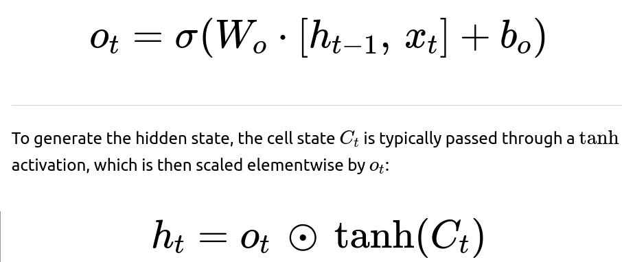
That allows the LSTM to selectively read aspects of its internal cell state when producing the hidden state for downstream consumption.
How the Gates Work Together

By design, each gate can be tuned during training through backpropagation. If the forget gate, for instance, consistently learns to keep certain components near 1.0 in tasks that require retaining older information, the LSTM cell state will effectively “remember” those components indefinitely. If certain components of the cell state are shown to be irrelevant, the LSTM can quickly drive the forget gate to near 1 for them, effectively removing them. Likewise, the input and output gates facilitate the introduction of new relevant signals and the controlled exposure of that state for downstream tasks.
In day-to-day practice, data scientists frequently rely on these gating mechanisms to handle more complex tasks such as language modeling and time-series predictions. They also tune hyperparameters, consider using multiple LSTM layers (stacked LSTMs), or even more sophisticated variants like GRUs if computational or memory constraints arise.
Implementation Example in Python
Below is a simple conceptual code snippet (in PyTorch-like pseudocode) that demonstrates how an LSTM step might be done manually. This can help illustrate the interplay of the forget, input, and output gates.
import torch
import torch.nn as nn

class ManualLSTMCell(nn.Module):
    def __init__(self, input_size, hidden_size):
        super(ManualLSTMCell, self).__init__()
        self.input_size = input_size
        self.hidden_size = hidden_size

        # Weights for forget, input, output gates and candidate cell
        self.W_f = nn.Linear(input_size + hidden_size, hidden_size)
        self.W_i = nn.Linear(input_size + hidden_size, hidden_size)
        self.W_o = nn.Linear(input_size + hidden_size, hidden_size)
        self.W_c = nn.Linear(input_size + hidden_size, hidden_size)

    def forward(self, x, h_prev, C_prev):
        # Concatenate input and previous hidden state
        combined = torch.cat((h_prev, x), dim=1)

        # Compute forget, input, candidate, output
        f_t = torch.sigmoid(self.W_f(combined))
        i_t = torch.sigmoid(self.W_i(combined))
        o_t = torch.sigmoid(self.W_o(combined))

        C_tilde = torch.tanh(self.W_c(combined))

        # Update cell state
        C_t = f_t * C_prev + i_t * C_tilde

        # Compute new hidden state
        h_t = o_t * torch.tanh(C_t)

        return h_t, C_t

# Example usage
batch_size = 2
input_size = 3
hidden_size = 4

lstm_cell = ManualLSTMCell(input_size, hidden_size)

# Initial hidden and cell states
h_prev = torch.zeros(batch_size, hidden_size)
C_prev = torch.zeros(batch_size, hidden_size)

# Random input
x = torch.randn(batch_size, input_size)

h, C = lstm_cell(x, h_prev, C_prev)
print("New hidden state:\n", h)
print("New cell state:\n", C)

Maintaining Long-Term Information

Selectivity in what to forget and what to retain is vital for tasks where not all historical information is valuable. This gating approach allows the LSTM model to selectively purge or keep memory, effectively dealing with the memory capacity problem that plain RNNs have.
Below are deeper explorations and potential follow-up questions that typically come up in a FANG-level interview scenario.
What problems in standard RNNs does the LSTM architecture solve?
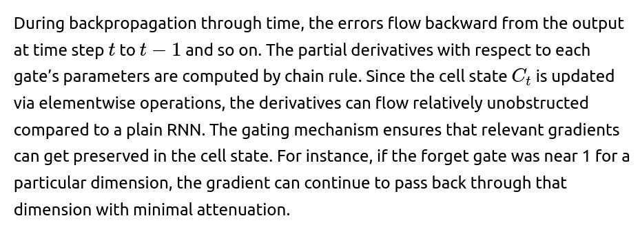
Standard RNNs suffer from vanishing or exploding gradients when sequences become long. This occurs because the gradients must flow back through many timesteps, and repeated multiplication with weights either diminishes or amplifies them too drastically. The LSTM architecture alleviates this by giving the model a more direct path for gradients to flow, primarily through the cell state which can carry signals forward with less repeated transformation.
LSTMs also allow the network to forget unneeded information and selectively add new information at each step. This is achieved by the learned gating mechanism that specifically zeroes out or reduces the magnitude of certain components of the memory (cell state) while amplifying or preserving the more relevant components.
How do the sigmoid and tanh activations in an LSTM cell affect its performance?
Sigmoid gates, which produce values between 0 and 1, serve as continuous “on/off” filters. They are used for all three gates because their outputs can be interpreted as a fraction of information to pass through (or forget). Tanh is typically used for the candidate cell state because it provides a range of negative to positive values while keeping them bounded. This helps stabilize training, because the cell state cannot grow unbounded when updating with newly introduced candidate information.
A key practical point is that if the sigmoid saturates (for instance, if the input to the sigmoid is very large in magnitude, leading to outputs near 1 or 0), training can slow down. Proper initialization, careful choice of learning rates, or techniques like layer normalization or initialization of biases (e.g., the forget gate bias being positive) can help mitigate these issues.
How do we interpret the cell state and the hidden state physically in the LSTM cell?
The hidden state is generally interpreted as the network’s “working output,” used directly in computations or passed to subsequent layers. The cell state can be viewed as the long-term memory store that flows through time steps with relatively minimal transformation, updated only through multiplication and addition as regulated by the gates. The cell state is often conceptualized as “internal memory,” while the hidden state is the current representation that the LSTM exposes to the outside world.
Why is the forget gate so important?
The forget gate is key to dealing with real-world sequence tasks where older inputs may no longer be relevant. Without the forget gate, the LSTM might accumulate irrelevant or outdated information indefinitely, leading to capacity saturation and inefficient training. The forget gate enables the LSTM to reset portions of its memory, preventing the model from being cluttered by stale data.
In the original LSTM formulation, the forget gate was actually introduced slightly later (the original design used a constant of 1.0 for forget gate, effectively never forgetting). The addition of the forget gate was a major improvement because it provided an explicit mechanism to discard information, which further stabilized training and improved performance in tasks requiring variable memory retention spans.
How would you initialize the bias terms for the forget gate?
A commonly used trick is to initialize the forget gate bias to a small positive number (like 1.0 or 2.0). This initial positive offset makes it more likely (at the start of training) that the network will retain information longer and not forget prematurely. Over time, if forgetting is beneficial, the network can learn to set those forget gates to lower values. This approach can improve training stability, particularly in tasks where longer-term dependencies are important.
Are there tasks where a basic RNN can outperform an LSTM?
In principle, if the sequences are very short, or if the relevant information is contained only in very recent timesteps, a basic RNN might perform adequately and train faster. In practice, LSTMs (or GRUs) often outperform basic RNNs in most tasks involving sequential data of non-trivial lengths. There can be rare corner cases in very short contexts or highly optimized GPU kernels for simple RNNs where performance differences might tilt slightly in favor of simpler architectures, but for the majority of real-world sequence tasks, LSTMs are superior due to their gating mechanisms.
What happens if the output gate is set to 1 at all times?

How do you handle exploding gradients in LSTM training?
One common strategy is gradient clipping, where gradients are scaled down if their norm exceeds a certain threshold. This ensures that large gradient updates do not cause the parameters to take extremely large steps, preventing instability in training. Another method is to carefully initialize weights to avoid large initial expansions. Using techniques like orthogonal or Xavier initialization for recurrent weight matrices can also help.
How does the LSTM backpropagate errors through gates?
How does an LSTM decide what to forget vs. what to keep?
This decision emerges from training data and the backpropagation learning process. The forget gate’s parameters will adapt in a way that, given the loss signal, the model learns to drop or retain certain signals in the cell state. Over time, it adjusts its weights to minimize the overall training (or validation) loss, effectively learning patterns about which parts of the sequence are important and which are not. The same applies to the input and output gates. These gating behaviors are not hard-coded; they are learned end-to-end from the dataset and the tasks the LSTM is solving.
How do you extend LSTMs to bidirectional processing?
In a bidirectional LSTM, one LSTM processes the sequence in the forward direction, while another LSTM processes it in reverse. The hidden states from both directions are typically concatenated at each time step to form the final output. This allows the network to incorporate context from both past and future. For tasks like text classification or named entity recognition, having bidirectional context can significantly boost performance. The gating mechanisms are the same, but each LSTM sees the data in opposite directions. The final output at each time step is constructed by combining both sets of hidden states.
How do we handle very long sequences where an LSTM might still struggle?
Though LSTMs are significantly better than standard RNNs at capturing long-range dependencies, extremely long sequences can still cause difficulties. Some strategies include truncated backpropagation through time, hierarchical or chunk-based processing of sequences, or using attention mechanisms (leading to Transformer-based models). Another approach is to consider memory-augmented networks or external memory modules. However, in many practical tasks, LSTMs remain quite powerful and are still widely deployed.
How does the dimension of the hidden state affect performance?
A larger hidden state dimension increases the model’s capacity to store and process information. This can improve performance if the task is complex or requires a lot of memory. However, it also increases computational cost and the potential for overfitting if the dataset is not sufficiently large. Balancing hidden size with dataset size and computational constraints is a recurring theme in deep learning architectures. Validation performance is often used to guide the choice of hidden state size.
Are LSTMs still widely used despite the popularity of Transformers?
Yes, they are still used in various production systems for tasks such as streaming data, time series forecasting, and embedded devices where the overhead of large Transformer-based models might be impractical. While Transformers can replace LSTMs in many NLP tasks, LSTMs still remain relevant because they often require fewer parameters, can be more memory-efficient for certain tasks, and remain robust solutions for streaming or on-device scenarios.
How do these three gates improve gradient flow compared to simpler RNNs?
By allowing the cell state to flow largely unimpeded (just multiplied by the forget gate and updated with input gate), the LSTM design provides a path for gradients to pass back through many time steps without being multiplied repeatedly by potentially unstable recurrent weights. The gating also ensures that irrelevant signals don’t get amplified or repeated ad infinitum, and can be quickly forgotten if needed.
When the gating parameters push the forget gate toward 1 for some components, those components can remain in the cell state over many time steps, carrying information forward. The derivative through a multiplication by near-1 is stable, letting gradient updates remain significant. This addresses the vanishing gradient problem, one of the main issues with naive RNNs.
How would you adapt an LSTM for multi-dimensional data, such as images?

How does the cell state combine old and new information?
Mathematically, the cell state at time t is:

How do LSTMs compare to GRUs?
Gated Recurrent Units (GRUs) are a streamlined alternative. They combine the forget and input gates into a single “update gate,” and they also merge the cell and hidden states into one. GRUs are simpler and often train slightly faster or require fewer parameters while still retaining a robust ability to capture long-term dependencies. LSTMs, on the other hand, can be more flexible for certain tasks because they separate the forget and input mechanisms, which can allow them to more finely control what gets added or removed from the cell state. In practice, both LSTMs and GRUs are widely used; the best choice often depends on empirical performance for the specific task.
Can an LSTM completely avoid the vanishing gradient problem?
LSTMs significantly reduce the vanishing gradient problem by providing a more direct path for gradient propagation. However, they do not entirely eliminate it, especially for extremely long sequences or if other architectural or training issues arise. In practice, though, LSTMs make it feasible to handle sequences of much greater lengths than what was possible with basic RNNs, which is why they became so dominant in sequence modeling tasks prior to the Transformer revolution.
What if the input gate is always 0?
If the input gate remains 0, the model does not add any new information into the cell state. Over time, the cell state would primarily rely on whatever was introduced before the gate locked at 0. This situation would severely limit the model’s capacity to learn from new inputs. During training, the model would quickly discover that a perpetually 0 input gate is detrimental unless the data distribution is extremely peculiar. Typically, the network will learn to open or partially open the input gate to integrate relevant new signals.
What if the forget gate is always 1?
If the forget gate is always 1, nothing is ever removed from the cell state. The cell state might accumulate irrelevant or noise-like information over time, or saturate if the input gate also frequently adds new information. This can hinder the capacity to differentiate relevant from irrelevant historical contexts. Training usually ensures that the forget gate doesn’t remain locked at 1 if there is reason to remove older memory.
Is there a scenario where LSTMs are less suitable?
For tasks with extremely large context windows—like very long documents or multi-day time series with many thousands of steps—LSTMs can still find it challenging. Transformers with attention mechanisms often handle such tasks more gracefully, because attention can theoretically access any position in the sequence directly without going through all intermediate steps. LSTMs also process data sequentially, making them less parallelizable for GPU-based acceleration compared to Transformers. However, LSTMs still shine for moderate sequence lengths and resource-limited scenarios.
Could we remove the output gate from an LSTM?

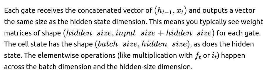
How do the gates change the shape or dimensionality of the data?
Could LSTMs handle non-numeric or highly structured data?
Yes, so long as the data can be transformed into a sequence of numeric embeddings. For example, text is commonly turned into word or subword embeddings, which an LSTM can process. For structured data, we typically flatten or embed the features each time step. Where LSTMs struggle is with data that has complex dependencies and doesn’t naturally fit a single sequence dimension. That’s why for images or videos, we often adapt them into convolutional LSTMs or simply switch to architectures like 3D CNNs or Transformers with spatiotemporal attention.
How do you usually initialize LSTMs in frameworks like PyTorch?
Modern frameworks provide default initializations (often uniform or glorot/uniform) for LSTM weight matrices. For stability, especially for forget gate biases, some developers manually set the forget gate bias to a positive value. One approach in PyTorch is to iterate through the named parameters of an LSTM layer, identify which part corresponds to the forget gate’s bias, and add a constant offset:
for name, param in lstm.named_parameters():
    if "bias_f" in name:
        nn.init.constant_(param, 1.0)
This ensures that initially the LSTM starts off by retaining more memory, which can help on tasks that need longer context.
Do LSTMs always require gating signals at every timestep?
Yes. At every time step, the forget, input, and output gates are computed anew. They control the flow of information at that time step. The gates can adapt from moment to moment, allowing the network to respond dynamically to the evolving sequence. This adaptability is precisely what makes LSTMs so powerful for sequential tasks.
How do LSTMs handle zero-padding of sequences?
When dealing with variable-length sequences, one approach is to zero-pad them to a uniform length and use a masking mechanism so that computations on padded steps do not affect the hidden or cell states meaningfully. In frameworks like PyTorch, you might use “pack_padded_sequence” and “pad_packed_sequence” to efficiently process batches of variable-length sequences. The LSTM then effectively ignores the padded parts once it knows how long each sequence is. Alternatively, you can process each sequence individually, but that’s less efficient.
How do LSTM gates decide how much context from the past is relevant for the future?
In a data-driven manner. During training, if retaining certain memory leads to a lower loss, the LSTM will adjust the forget gate parameters to keep that memory across time steps. If introducing certain new signals in the cell state helps predictions, the input gate parameters will shift to allow that new info in. Over time, the gating parameters converge to a configuration that best leverages relevant historical context while discarding unhelpful or distracting memories. This is learned through backpropagation and is not explicitly hand-coded.
What is the significance of each gate’s bias term?
Each gate has a separate bias term so it can shift the output of the linear combination before the sigmoid or tanh activation. In the forget gate, for instance, the bias can be initialized to a positive value to encourage retention initially. Bias terms allow the gate outputs to be nonzero even if the weighted sum of the inputs is zero. They provide the model with added flexibility to decide how to process input data, especially early in training before the weights converge.
If we have an extremely large training set with complex temporal dependencies, can we stack multiple LSTM layers?
Yes, a stacked or deep LSTM has multiple layers of LSTM cells. The hidden state from one LSTM layer becomes the input to the next layer at each time step. This can allow the network to build up a hierarchy of temporal representations. While it often improves representational capacity, it also increases computational cost and the risk of overfitting. Techniques like dropout can be applied between LSTM layers to help regularize the model.
How can we visualize the forget, input, and output gate activations?
You could log the gate values at each time step for a small batch of data. By plotting them over time, you can see how the model “turns on” or “turns off” certain components of the hidden state. This can yield insights into how the model is processing sequences. Sometimes, you might see that the forget gate remains high for certain timesteps until a key event occurs, and then the model drops that memory. Such visualizations can be instructive in debugging or understanding LSTM behavior.
Could we add more gates to an LSTM?
In principle, yes, you could design advanced gating mechanisms. Over the years, researchers introduced variants like peephole connections (where gates can directly see the cell state) or additional gates to handle special tasks. However, the standard three-gate LSTM design remains the most widely used and robust for a broad range of applications. Adding more gates can overcomplicate training unless there’s a compelling reason to do so.
Why do we multiply the cell state by the forget gate instead of adding it?
Multiplication by a value in (0,1) acts like a filter or a gate, selectively attenuating or retaining information. Addition would integrate new signals but wouldn’t provide the direct mechanism for discarding information in a multiplicative way. Using addition for forgetting might require carefully balancing negative and positive components, which can be less intuitive. The multiplicative interaction ensures a dimension-by-dimension control, making it straightforward to zero out (or partially zero out) memory content.
How do these gates compare to attention mechanisms in Transformers?
Attention mechanisms also decide how to weigh different parts of a sequence but do so by computing pairwise attention scores rather than gating a persistent cell state. LSTMs rely on a hidden state plus an internal cell state regulated by gates, while Transformers rely on explicit pairwise attention across all positions in the input. Both accomplish the broad goal of selectively focusing on relevant information, but they do it in very different ways. The gating in an LSTM is more local and unrolled over time, whereas attention is typically a global operation across the entire sequence for each step.
Why do LSTMs use tanhtanh instead of ReLU for the cell updates?
tanh keeps values bounded between −1 and 1, which can help stability when the cell state is updated. If you used ReLU, the state could grow unbounded, potentially causing exploding activations or complicated gradient behavior. That said, some variants of LSTM do experiment with ReLU or other activation functions, but the standard formulation uses tanh.
Why do we use separate weight matrices for each gate?
Each gate has a distinct function (forget, input, output). Having separate weight matrices allows the model to learn distinct transformations for each of these functionalities. If they shared weights, it would constrain the gating behaviors to a single learned representation, possibly limiting expressiveness. Each gate needs specialized parameters to best fulfill its role in regulating information flow.
What happens if the forget gate is always near zero?
That would mean the model is frequently discarding old memory at every time step. It would effectively behave like a short-term memory, resembling a simpler RNN where the hidden state is quickly overwritten by new inputs. This can be harmful if the task requires remembering something from much earlier in the sequence. In practice, you might see that the LSTM’s forget gate is near zero for irrelevant states but near one for important features.
How do you tune an LSTM’s hyperparameters?
Common hyperparameters include:
Hidden size (dimension of hidden and cell states)
Number of layers in a stacked LSTM
Dropout rate between layers
Learning rate and optimization method
Sequence length or truncated backpropagation length
Batch size
Weight initialization schemes (especially for forget gate bias) You typically adjust these based on validation performance or domain knowledge. The size of the dataset and the complexity of the task drive many of these decisions.
Could we store multiple distinct pieces of information in the cell state?
Yes, the cell state is a vector, so different dimensions can hold different pieces of information. The gating mechanisms operate on each dimension independently. The LSTM can learn to store separate features of the sequence in separate components of the cell state, adjusting gates so that each component is retained, updated, or forgotten as needed.
Is there a known theoretical limit to how far back an LSTM can remember?
In principle, if the forget gate remains near 1 for some dimensions, and there’s no destructive overwrite via the input gate, the cell can carry those dimensions indefinitely. In practice, numeric precision, architectural constraints, and noise from training data can erode perfect memory over extremely long sequences. However, LSTMs certainly extend the feasible memory capacity far beyond that of vanilla RNNs.
How do LSTMs handle noisy inputs?
The gating system can learn to filter out or forget noise if it doesn’t help minimize the overall loss. The input gate, for instance, might remain near zero if an input is uninformative or contradictory. Over repeated training, the network can learn to reduce the effect of noisy signals, though this depends on having enough data and meaningful patterns to isolate noise from relevant signals.
Are there improvements upon LSTM gating mechanisms?
Numerous variants exist, including peephole LSTMs (which feed the cell state into the gates), GRUs, and others. Yet the standard LSTM design remains a cornerstone. More significant changes bring us into the domain of attention-based Transformers, which have largely become the default in NLP. Still, the gating idea remains at the heart of many modern architectures that strive to handle temporal or sequential data.
Each of these points shows how the forget gate, input gate, and output gate collaboratively ensure that the LSTM can maintain long-term information and decide what to forget, add, or expose at any given time step. This powerful combination of gating is exactly what sets LSTMs apart from simpler recurrent architectures, enabling them to remember patterns over much longer contexts and address some of the biggest limitations of vanilla RNNs.
Below are additional follow-up questions
How do LSTMs behave in real-time streaming data, and what specific design considerations or pitfalls arise in this context?
When using LSTMs in streaming applications (for instance, live sensor data, online user input, or real-time signal processing), you typically feed data into the network one time step at a time. The cell state and hidden state propagate forward, allowing the model to keep a running summary of recent history. A common pitfall is that real-time data can have concept drift, meaning data distributions shift over time. The LSTM might fail to adapt if it was trained on an earlier distribution. Potential solutions include:
Fine-tuning or re-training on new data as it arrives (online or incremental learning).
Using a windowing or chunk-based approach, periodically resetting the cell state to prevent stale information from accumulating.
Carefully monitoring memory usage and model latency. LSTMs process data sequentially, which can introduce latencies or limit throughput.
Edge cases arise when network throughput or latencies are tight. You must ensure that each LSTM step can handle the input rate without bottlenecks. In many real-time scenarios, memory constraints may also be a concern, as continuously storing large hidden states for many parallel streams can be resource-intensive. Balancing performance with resource limits is crucial.
What are the potential pitfalls of using teacher forcing when training LSTMs, and how can they be mitigated?
Teacher forcing is a technique where, at each time step in training, the ground truth output from the previous step is fed as input to the LSTM rather than the model’s own prediction. This accelerates convergence by providing the model with correct context. However, in real-world inference, the model receives its own predictions as inputs (especially in tasks like language generation). This discrepancy can cause “exposure bias”: the network never learns to recover from its own mistakes since it always sees perfect inputs during training.
Common mitigations include:
Scheduled sampling: gradually replace ground truth inputs with model predictions during training, increasing the fraction of predicted inputs over time.
Mixed teacher forcing strategies: occasionally feed the model’s own predictions even early in training to help it learn to handle noisy or incorrect inputs.
Techniques like beam search or sampling-based training that expose the model to potential errors.
A subtle pitfall is that teacher forcing can produce artificially good results during training but degrade severely at inference time. Ensuring that the training procedure aligns with how the model is used at inference is key.
How do LSTMs handle missing data or irregular time intervals in time-series tasks, and what strategies exist to improve performance?
Real-world time series data often has missing points or events that do not arrive at perfectly uniform intervals. Standard LSTM designs assume regularly spaced timesteps. If the data is sporadic or has gaps, naive feeding of zeros or placeholders can confuse the gating mechanisms, since the LSTM might interpret those artificial placeholders as genuine features.
Common strategies:
Imputation methods: fill in missing values based on domain knowledge or interpolation. While simple, it can introduce bias if the imputation model is poor.
Additional inputs to the LSTM that encode the “delta time” between arrivals, allowing gating mechanisms to learn patterns in how time gaps affect state updates.
Masking techniques: maintain a mask vector that indicates which inputs are missing or invalid at each time step. This mask can inform the input gate to ignore certain fields.
Using a specialized model like a GRU-D or T-LSTM that explicitly incorporates missingness indicators into the gating or updates. These variants learn how much to decay the hidden state as time gaps increase.
A pitfall is that naive approaches (like simply ignoring timesteps) can break the sequential assumption. Properly modeling the irregular intervals ensures the gating logic reflects the real temporal dynamics rather than artificial placeholders.
Could you use reinforcement learning with an LSTM policy, and are there any special considerations?
Yes, LSTM networks are widely used as policy or value-function approximators in reinforcement learning (RL) tasks, especially in partially observable environments where the agent cannot rely on a single observation to make decisions. The hidden state from the LSTM can help the policy “remember” relevant events across multiple timesteps.
Special considerations:
If episodes are long, naive backpropagation through time might become expensive or unstable. Truncated backprop through time is common.
Initialization of hidden states at the start of each episode is typically zeroed out, but in continuous or infinite-horizon tasks, you may carry forward states across sub-episodes.
Exploration strategies (like epsilon-greedy or policy gradient) can interact with gating behaviors. If the gating never sees diverse states because exploration is insufficient, it may fail to learn robust long-term memory.
The credit assignment problem can become more severe when there are long delays between actions and rewards. The gating mechanism can help, but hyperparameters may need careful tuning to ensure stable training.
A pitfall is partial observability, where the gating system might need to rely heavily on past states for crucial information. If the environment changes drastically, the LSTM’s memory might hamper adaptation unless you reset or retrain the memory.
How do you incorporate attention with LSTMs if you want a hybrid approach, and what edge cases can arise?
Attention mechanisms can be combined with LSTMs by letting the hidden state at each time step attend to a range of contextual embeddings or previous hidden states. A common scenario is in sequence-to-sequence models (like neural machine translation) where the encoder is an LSTM, and a decoder LSTM uses an attention mechanism to focus on different parts of the encoder output at each step.
Key steps in a hybrid approach:
The encoder LSTM processes the input sequence into hidden states.
For each timestep in the decoder LSTM, the network computes attention weights over the encoder states.
The attention-weighted context vector is then used as an additional input to the decoder, informing the gating about which encoder positions to emphasize.
Potential edge cases:
The LSTM gating might become over-reliant on the attention context and fail to properly use its own hidden state for local predictions, leading to suboptimal learning of internal representations.
If the attention distribution saturates (always focusing on a single token or a small subset), you lose the broader context. Balancing gating signals and attention coverage is essential.
Handling extremely long sequences might still pose challenges, as the complexity grows with sequence length for attention-based computations.
What are some memory and computational cost considerations in large LSTM deployments, and how do you address them?
Large LSTMs, especially with high hidden dimensionality or stacked layers, can be computationally expensive. Each gate involves a matrix multiply that depends on both the hidden size and input size. Memory usage grows proportionally with the number of parameters (and any intermediate states stored for backprop). As the batch size or sequence length increases, so does the computational overhead.
Potential solutions:
Model pruning or parameter sharing to reduce the parameter count in gating (e.g., using techniques like matrix factorization for gate weight matrices).
Mixed-precision training (float16/32) to reduce memory footprint while speeding up computation, provided hardware supports efficient half-precision operations.
Using optimized library kernels designed for RNNs (like CuDNN on NVIDIA GPUs) to maximize parallelization.
Layer normalization or grouped linear operations that can reduce overhead in some cases.
A subtle pitfall: if you reduce precision too aggressively or prune heavily, the gating behavior can degrade, losing the nuanced memory control that LSTMs rely on.
Can you apply weight tying with LSTMs in the same way as with Transformer language models?
Weight tying often refers to using the same weight matrix for the input embeddings and the output projection layer in language models, reducing parameter count. In principle, you can do something similar for LSTM-based language models, tying the embedding matrix and the softmax output matrix. This is sometimes referred to as “output embedding tie.” It saves parameters and can improve consistency between input and output token representations.
Potential pitfalls:
The dimension of the hidden state might not match the dimension of the embedding directly, necessitating additional projection layers or transformations.
You must ensure the gating computations themselves aren’t inadvertently changed. The forget, input, and output gate weight matrices typically remain separate.
If the hidden dimension is large, you might still have a mismatch with the vocabulary embedding dimension, leading to additional overhead for projection steps.
If done carefully, weight tying can significantly reduce the parameter footprint without harming performance, but it requires consistent dimensional setups and possibly an extra projection if the LSTM hidden size differs from the embedding size.
How do you quantify interpretability for LSTM gating, and are there ways to interpret or visualize the gating behavior for domain experts?
LSTMs are more opaque than simpler linear models because gating is dynamic, changing per time step. However, certain interpretability approaches exist:
Gate activation visualization: plot the forget, input, and output gate values across time for a given sequence to see how strongly or weakly the model is retaining or discarding information.
Feature attribution methods (e.g., integrated gradients, gradient-based saliency): measure how changes in input at a certain timestep affect the eventual output or gating decisions.
Cell state analysis: track how each dimension of the cell state evolves over time. If certain cell state dimensions strongly correlate with a known signal in the data, that dimension might be representing that feature.
A subtle pitfall is misinterpretation: while you might see that a certain gate’s activation is high at a certain step, it doesn’t necessarily imply a simple causal relationship. The gating behavior emerges from a high-dimensional optimization process. Domain experts may require additional context or partial correlation analyses to interpret LSTM gating in a meaningful way.
How do you handle partial gradients or truncated backpropagation through time (BPTT) effectively with LSTMs?
In practice, training on very long sequences can be intractable if you propagate gradients through the entire sequence. Truncated BPTT limits how far back in time you flow gradients. For instance, you might backprop through only 20 timesteps at a time, then detach the computational graph from older timesteps.
Implications:
This can reduce memory usage and computational cost, making large-scale training feasible.
The model might lose some long-term context during training if the relevant signals lie beyond the truncated window. However, the gating can still carry partial information, and if the network sees overlapping segments, it can learn to store vital aspects in the cell state.
A potential edge case: if the sequence has critical dependencies spanning more than the truncated length, the model could fail to learn those dependencies robustly. You might need a careful choice of truncation window or specialized training curriculum that exposes the network to longer sequences when feasible.
Are there advanced optimization strategies or scheduling that specifically help LSTM training?
Yes, beyond standard optimizers like Adam or RMSProp, there are specialized tweaks:
Learning rate warm-up: gradually increasing the learning rate from a small value can help stabilize early gating updates, especially if the forget gate is biased high.
Gradient noise injection: adding small random noise to gradients can prevent the gates from saturating too quickly or dropping essential signals.
Gradient clipping by global norm or by specific gate norms can help avoid instabilities in gating operations.
A subtle pitfall is that over-aggressive clipping or advanced scheduling can lead to underfitting if the network never sees strong enough gradient signals. Finding the sweet spot often requires empirical tuning. Also, if your gating saturates too quickly, scheduling a slower learning rate initially may help the network maintain differentiable gate outputs.
Could we train LSTMs in low precision (e.g., half precision or mixed precision), and what are the pitfalls?
Mixed-precision training is commonly used to accelerate deep learning models and reduce memory consumption. LSTMs can benefit from this, but special attention is required:
Gating calculations involve sigmoid and tanh operations that can be sensitive to numerical rounding. Extreme inputs might saturate the sigmoid faster if precision is too low.
The cell state may accumulate small numerical errors over many timesteps, potentially impacting the model’s ability to store information accurately if the accumulations are not carefully handled (e.g., by maintaining a higher-precision master copy of the weights).
Proper scaling of gradients and intermediate activations is vital to avoid overflow or underflow.
Overall, frameworks like PyTorch’s autocast can manage these pitfalls, but you should monitor for divergence or gate saturation more closely when using half precision.
What is the role of the activation function for the gating signals if we replaced sigmoid with something else?
Sigmoid is conventionally used because it produces a value in (0,1), making it intuitive as a gating coefficient. If you replaced it with, say, a hard-sigmoid or ReLU variant, you would alter the gating mechanism:
A ReLU gate can’t produce negative values and could let large positive values pass through, losing the bounded nature that is central to LSTM gating.
A hard-sigmoid might be faster or more robust to saturation but is less smooth, potentially affecting gradient flow in borderline regions.
Swish or other parametric activations have been explored but are less common. They might provide slightly better gradient properties, but it’s not guaranteed.
Pitfalls:
The interpretability of gating as “fraction of information passed” may not be as direct if your gating function is unbounded or produces values outside (0,1).
Convergence behaviors may differ, requiring hyperparameter retuning.
Could we add skip connections or residual connections inside LSTMs, and why might we do this?
Yes. One approach is to let the cell state or hidden state at time t incorporate a residual-like skip from t−1. Standard LSTM already has a partial skip since the cell state is passed forward with a simple multiplication and addition. However, you can add additional skip or highway connections to facilitate gradient flow and encourage better feature reuse across timesteps or layers.
For instance, in stacked LSTMs, you might feed the hidden state from layer k−1 not just to layer k, but also skip to layer k+1. This can help alleviate vanishing gradients or improve training speed.
Pitfalls:
Too many skip connections can lead to overfitting or hamper the gating logic by overshadowing the LSTM’s carefully regulated memory updates. The model may start to rely on skip pathways rather than the gates, making the gating less critical or underutilized.
Implementation complexity: custom solutions can be error-prone unless carefully tested.
Is it beneficial to combine LSTMs with CNNs for tasks like speech recognition or NLP, and how?
Combining CNNs and LSTMs can capture both local structure (via convolution) and long-term dependencies (via recurrent gating). In speech recognition, for example, a CNN front-end can extract local acoustic features from spectrogram patches, and an LSTM back-end can track temporal patterns. In NLP, convolution layers can quickly capture local n-gram features, while an LSTM can model global context.
Potential pitfalls:
Aligning the time dimension between the CNN output and LSTM input sometimes requires careful reshaping or pooling strategies.
Large convolutional feature maps can inflate memory usage before feeding into an LSTM. Designing the architecture to reduce spatial or temporal dimensions before the LSTM helps.
Overfitting if the combined model is too large. Techniques like dropout or batch normalization might be necessary at the convolution or LSTM layers.
How do LSTMs scale to large vocabularies in language modeling tasks, and are there gating or memory issues that arise?
When modeling natural language with very large vocabularies, an LSTM typically maintains the same gating computations regardless of vocabulary size (the gating dimension depends on the hidden size, not the vocabulary size). However:
The embedding layer and the final output projection can become huge if the vocabulary is large. While the gating itself remains unaffected dimensionally, the overall model size can become unwieldy.
Softmax computations can be expensive, leading to the need for sampling-based or hierarchical softmax approaches for large-vocabulary setups.
The gating might remain stable, but the LSTM is more prone to overfitting if the vocabulary is huge and the hidden layer is large. Regularization (dropout, weight decay) is crucial.
An edge case is subword-based or byte-pair encoding approaches, where you reduce the effective vocabulary. This can alleviate some memory burdens and might lead to more effective gating because the model sees subword sequences, giving it finer control over morphological or partial-word memory.
What are the typical ways to reduce overfitting in LSTM models beyond gating, and how might they interact with the gates?
Beyond the inherent gating structure, LSTMs often employ:
Dropout: typically inserted on the inputs, outputs, or even recurrent connections. However, naive dropout on recurrent connections can disrupt memory. Techniques like variational dropout or locked dropout maintain the same dropout mask across timesteps to preserve gating consistency.
Weight decay: a small penalty on the magnitude of the weights can help the gates avoid saturating at extremes.
Early stopping: monitor validation performance and stop training if performance declines.
Data augmentation: in sequence tasks (e.g., text generation), artificially augmenting data might be trickier than in vision tasks, but for audio or sensor data, you can add noise or random time shifts.
A subtle pitfall is that if dropout is too high on the recurrent connections, the cell state transitions become noisy, which might harm long-term memory retention. The gating could become erratic, preventing stable memorization.
Could we prune or compress the LSTM gating parameters to reduce model size, and what effect might that have?
Yes, techniques like magnitude-based pruning or structured pruning can be applied to gating parameters. One approach might prune entire units in the hidden state, effectively removing certain dimensions of the cell and gating. This can significantly reduce the parameter count and memory footprint.
Potential pitfalls:
Over-pruning can degrade the model’s ability to store or forget critical information. The gating might no longer function properly for nuanced contexts if too many dimensions are removed.
After pruning, you may need to fine-tune the network to restore performance. The gating parameters might require careful rebalancing post-pruning.
Unstructured pruning can lead to irregular memory access patterns that might not improve actual runtime on certain hardware, though the theoretical parameter count is lower.
Can we incorporate gating on multiple timescales within a single LSTM cell?
Some variations of LSTMs introduce multiple cell states (or nested gating) to capture information at different timescales. Each sub-cell might have its own forget and input gates, allowing one sub-state to capture long-term patterns while another focuses on short-term details.
Benefits:
A single LSTM cell can adapt to very different temporal patterns. One dimension might be very slow-decaying, while another dimension updates rapidly.
This approach can be more parameter-efficient than stacking multiple LSTM layers or building separate networks.
Pitfalls:
Training complexity. The more gating layers within the cell, the greater the risk of gating saturations or conflicting signals.
Harder to interpret. With multiple gating streams, diagnosing which timescale is controlling which feature can be challenging.
What specific data preprocessing steps might help an LSTM gating mechanism be more effective?
Proper data preprocessing can help gating:
Normalizing or scaling input features so that they fall within a range that does not saturate sigmoids or tanh. Extreme values can push gates to 0 or 1 too frequently.
Denoising or smoothing signals, especially in time-series tasks with high-frequency noise, so gating doesn’t get triggered erroneously by random spikes.
Tokenization strategies in NLP to reduce out-of-vocabulary words and produce more stable embeddings.
Sequential bucketing for data with varying lengths, ensuring that each batch is roughly the same sequence length, preventing the LSTM from toggling frequently between short and long contexts.
Pitfalls:
Over-normalizing can remove meaningful magnitude cues. If certain features rely on large absolute values to signal events, gating might lose that signal.
Using an overly aggressive smoothing method may wash out abrupt but critical temporal changes. The gating might then learn an averaged, less responsive pattern.