
ML Interview Q Series: Markov Chain Analysis of Win Probability in a Two-Round Lead Game
Browse all the Probability Interview Questions here.
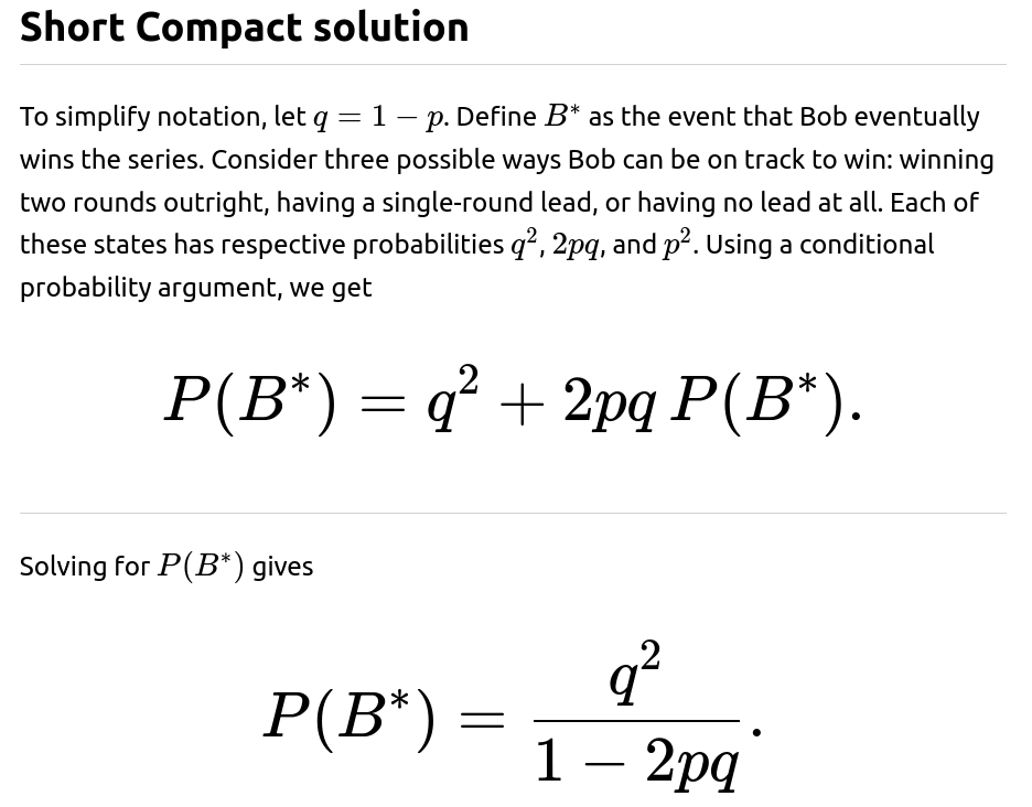
Alice and Bob repeatedly play rounds of a game. Each round is won by Alice with probability p and by Bob with probability 1−p. They continue until one of them is ahead by two rounds. What is the probability that Bob ends up winning the entire series?
Comprehensive Explanation
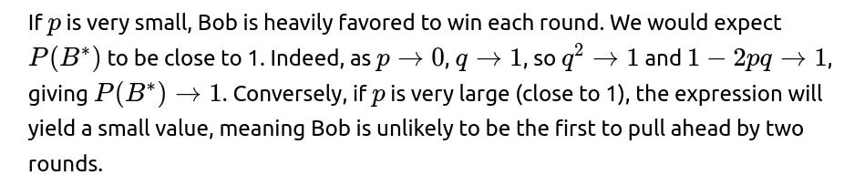
The series continues until the absolute difference in the total number of rounds won by each player reaches two, meaning one player is exactly two ahead of the other. Since Alice wins each round with probability p and Bob wins each round with probability q=1−p, the process can be viewed as a Markov chain or a one-dimensional random walk on the difference in the number of wins.
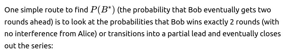
When analyzing Bob’s overall probability of success, we look at small “transient” states. Let’s name a few key states according to Bob’s advantage over Alice:
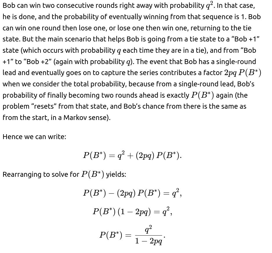
Bob leads by 0 rounds (the score is tied). Bob leads by 1 round. Bob leads by 2 rounds, at which point Bob has won the entire series.
If Bob is at a lead of 2 rounds, he has effectively captured the series, so his probability of winning from that point is 1. If the game transitions to Bob having a lead of 1 round, we treat it as an intermediate state where Bob has not yet won but is on the path that can lead to winning. A similar situation exists if the game transitions to the tie state (lead by 0), which can occur multiple times until eventually either Bob or Alice pulls ahead by 2.
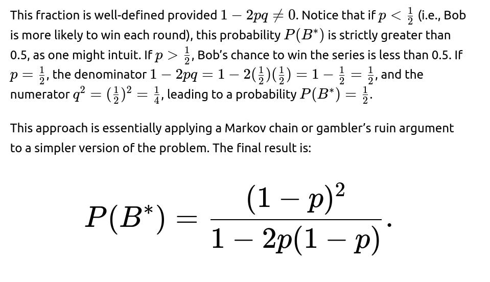
What if p=0.5?
If p=0.5, then q=0.5 as well. Plugging in those values:
This is an intuitive outcome: if both have equal chance per round, each player has an equal 50% shot to be the first to go two rounds ahead.
Could this be solved using a gambler’s ruin formulation?
Yes. One can frame it as a random walk representing the difference in total wins between Bob and Alice. The difference moves +1 in Bob’s favor with probability q and −1 in Alice’s favor with probability p. The boundaries are +2 and −2. We only care about the probability of hitting +2 before −2. This is precisely the gambler’s ruin scenario where each step is won or lost with certain probabilities. Standard gambler’s ruin formulas yield the same result.
How can we simulate this numerically?

import random

def simulate_bob_win_probability(p, num_simulations=10_000_00):
    q = 1 - p
    bob_wins = 0
    for _ in range(num_simulations):
        # Start with 0 difference (Bob's wins - Alice's wins)
        diff = 0
        while abs(diff) < 2:
            if random.random() < p:
                diff -= 1
            else:
                diff += 1
        if diff == 2:
            bob_wins += 1
    return bob_wins / num_simulations

estimated_probability = simulate_bob_win_probability(0.3)
print("Estimated Probability Bob Wins:", estimated_probability)
This code simulates many trials, each time tracking the difference in score until it reaches +2 (Bob leads by 2) or −2 (Alice leads by 2).
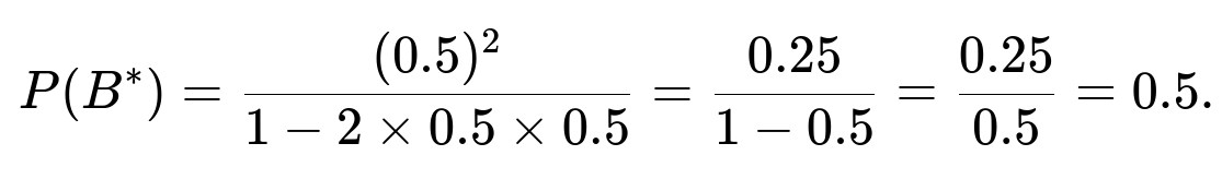
What happens if 1−2pq=0?
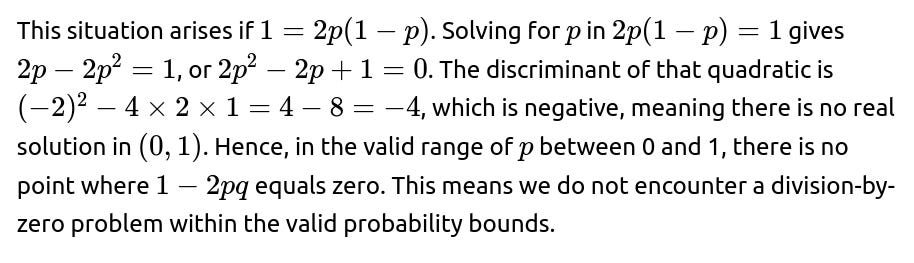
How does intuition align with the formula?
Could the approach be extended to a lead of more than two?
Yes, one can extend this to a situation where the game ends when one player is ahead by k rounds. The difference would then be a random walk with boundary states at +k (Bob wins) and −k (Alice wins). The gambler’s ruin analysis extends naturally, and the method of solving would be similar but with different boundary conditions. The approach would produce a more general formula for the probability of hitting +k before −k.
Is there a relationship to expected duration of the game?
Another possible question is how many rounds, on average, it takes before someone is ahead by two rounds. A general approach uses Markov chain techniques or can adapt gambler’s ruin formulas for expected hitting times. Such calculations typically involve solving systems of linear equations for mean hitting times or using well-known gambler’s ruin results. The main idea is to exploit the Markov property: from each state of the difference in wins, we set up an expectation equation in terms of the neighboring states, then solve.
How do we handle bias in real-world scenarios?
In practice, p might not be a fixed probability but could vary over time, or each round may not be independent. The basic derivation here uses independence and a constant probability for each round. If the probability shifts or if the rounds are correlated, a more complex model (such as a non-homogeneous Markov chain or a hidden Markov model) might be necessary. Data scientists often need to check stationarity and independence assumptions before applying this type of analysis in real-world settings.
Below are additional follow-up questions
How does the probability distribution of the score difference evolve over time?
One way to explore the problem is by looking at the distribution over all possible differences in score after each round, often referred to as the state distribution of a Markov chain. The difference in the number of rounds won by Bob versus Alice can be denoted as an integer state that starts at 0 and evolves according to:
With probability q=1−p, the difference increases by 1 (Bob wins that round).
With probability p, the difference decreases by 1 (Alice wins that round).
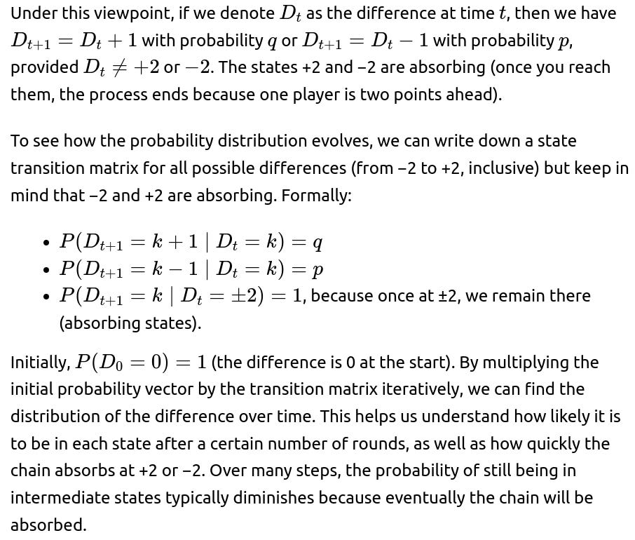
How can we systematically consider partial leads and their transition probabilities?
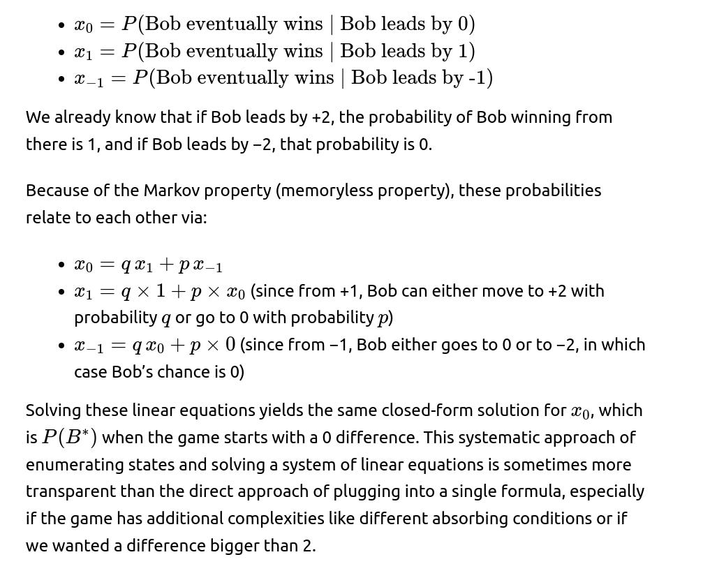
A more rigorous approach to partial leads begins by labeling each possible lead by Bob (e.g., Bob leading by 0, Bob leading by 1, Bob leading by −1, etc.). Then we write the probability that Bob eventually wins (i.e., ends up at +2) starting from each state. These unknowns can be denoted as:
What if a round can end in a draw?
In some games, there might be a small probability of a tie each round. Suppose that with probability r a round is declared a draw (nobody gains a point), and with probabilities p and q=1−p−r respectively, Alice or Bob gets a win. The ending condition is still that one player must be two points ahead.
In this scenario, the difference in scores still performs something akin to a random walk, but now there is a probability r that the difference remains the same in a given step. This modifies the transition probabilities:
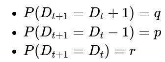
The states +2 and −2 remain absorbing. We can either solve it through a Markov chain approach or attempt to adapt gambler’s ruin arguments with an extra “stay still” probability. Typically, the presence of r>0 lengthens the time to absorption because draws keep the state from changing. The ultimate probabilities for Bob or Alice to end up two points ahead remain the same ratio as if one re-normalizes the jump probabilities p/(p+q) and q/(p+q), ignoring the draws. However, one must be cautious: the event of reaching +2 or −2 eventually might now depend on the chain being recurrent or transient if rr is large (especially in infinite state spaces). In the standard finite difference scenario from −2 to +2, the chain is still absorbing at ±2, so the probability distribution for Bob or Alice winning remains well-defined, though the time to absorption may increase due to repeated draws.
How do we handle the scenario of forced termination after a fixed number of rounds?
Sometimes practical constraints specify a maximum number of rounds, N, after which the game stops. If neither side is ahead by two at that point, another rule might decide the winner (e.g., whoever is currently leading, or a tiebreaker). In that case, the probability that Bob is two rounds ahead by the time we reach N is one part of the story, but if Bob is not two ahead (and Alice is not two ahead) when N is reached, the final decision might be made differently.
To account for this, we can modify the random walk to terminate after the $N$th step if the absorbing states (+2 or −2) have not been reached. The overall probability that Bob wins the tournament would then be:
Probability Bob is at +2 before or on round N, plus
Probability Bob is not at +2 (and neither is Alice at −2) by round N, but Bob is ahead by 1 (or tied, depending on the tiebreak rule), multiplied by the probability that Bob is declared the winner under that rule.
A Markov chain with absorbing states +2, −2, or “time out” after round N can be analyzed either by enumerating all paths or using the chain’s transition matrix truncated to N steps. In real tournaments, such constraints often exist, and it becomes a more complicated but still structured probability problem.
What is the role of symmetry or lack thereof?
In the standard scenario, the process is symmetric when p=q=0.5, and in that case, the chance for either player to be the first to +2 or −2 is 0.5. But in some settings, we could encounter an asymmetric game where Bob wins with probability q but the margin required for Bob might be different than for Alice—e.g., Bob needs only a 1-point lead to win, while Alice needs a 2-point lead. That breaks the symmetry entirely and changes the boundary conditions of the random walk. Instead of having absorbing states at +2 and −2, we might have absorption at +1 for Bob but −2 for Alice. Solving that scenario involves the same approach—setting up new absorbing boundaries and deriving the probability of hitting +1 before −2. The formula changes accordingly, and one typically ends up with a general gambler’s ruin expression for hitting +k (for Bob) before −m (for Alice).
A potential pitfall is incorrectly using the standard “2 lead” formula in a scenario that is not truly symmetrical. Overlooking differences in the threshold required for each player’s victory is a common source of error.
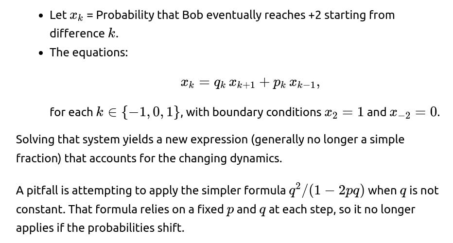
How would we deal with a scenario in which the probability of winning a round depends on the current score difference?
In certain realistic games, a trailing player might become more motivated, or a leading player might lose concentration or become overly confident, so that p (or q) is not constant but a function of the current difference. For example, if Bob is trailing, he might have a higher probability of winning the next round due to playing more aggressively.
To handle such a setting, we can still model it as a Markov chain, but the transition probabilities now depend on the state. For instance:
We then set up a transition matrix reflecting these state-dependent probabilities. The absorbing conditions remain the same: once you hit +2 or −2, the game is over. The system of linear equations or standard Markov chain absorption analysis can still be applied:
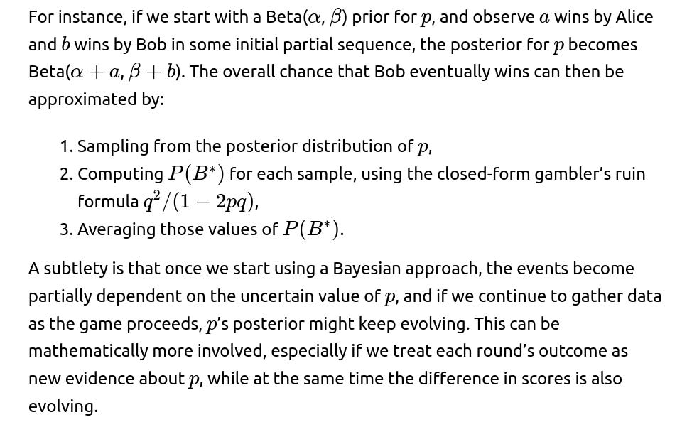
What if we observe the outcomes of initial rounds before deciding p?
In certain experiments or real-world scenarios, we might not know p upfront but want to infer it from observed data—for instance, the first few rounds’ outcomes—and then update our estimate of p as the game continues. This introduces a Bayesian perspective. We might place a prior on p (for example, a Beta distribution) and update it as we observe additional wins and losses. The probability that Bob ultimately leads by 2 can be integrated over the posterior distribution of p.
How might a “best-of” structure alter the analysis?
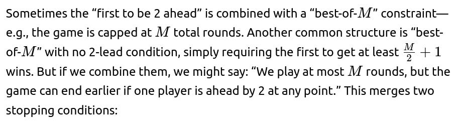
One player leads by 2 at any time (absorbing boundary in the difference).
We run out of rounds (M completed).
In that scenario, we must track both the difference in score and the number of rounds played. The state might be represented by (difference,round count), and the chain can be quite a bit larger to handle. A typical pitfall in analyzing such scenarios is failing to incorporate the “round count” dimension. Ignoring it might lead to miscalculations about how the probabilities unfold near the end of the M allowed rounds.
How does the variance in the duration of the game inform strategy?
From a practical standpoint, managers or players might care not just about the probability of winning but also how quickly the game is likely to resolve. Sometimes, if a tournament or environment imposes time constraints, it can be advantageous to know the distribution of how many rounds it typically takes before someone leads by 2.
A high variance in duration means the game can occasionally drag on for many rounds if the score difference oscillates around 0 or ±1 for a long time. In certain real-world competitions, such as tennis tiebreaks, a two-point lead is required, which can lead to extended deuce scenarios. Understanding the variance and expected length can guide scheduling or stamina-based strategies.
A subtle edge case arises if p≈0.5—the variance of the length can be quite large because the random walk is nearly symmetric, so it can hover around 0 or ±1 for many rounds. If p is extreme (close to 0 or 1), the series may end quickly on average, with either Bob or Alice quickly establishing a 2-point lead.