
ML Interview Q Series: Maximum Die Roll Probability: Using the Difference of Cumulative Probabilities
Browse all the Probability Interview Questions here.
18. A fair die is rolled n times. What is the probability that the largest number rolled is r, for each r in 1..6?
To deeply understand why this probability takes its well-known form, consider the experiment of rolling a fair six-sided die (faces numbered 1 through 6) exactly n times, each roll independently. We want the probability that the maximum (largest) outcome across all n rolls is exactly a specific value r, where r can be any integer from 1 to 6.
Fundamental Reasoning
One way to approach this is by thinking about two complementary events for any candidate largest value r: All the dice show values less than or equal to r. All the dice show values less than or equal to (r − 1).
If the largest value among the n rolls is exactly r, then certainly no roll is above r. So all rolls must be at most r. However, at least one roll must be r itself (otherwise the largest would be at most r − 1). Combining those two statements in a probability sense leads us to subtract the probability that all rolls are at most r − 1 from the probability that all rolls are at most r.
Mathematical Derivation
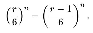
The probability that a single die roll is at most r is r/6, because each face is equally likely for a fair die, and there are r favorable outcomes out of 6 possible faces. For n independent rolls, the probability that each one of them is at most r is (r/6)^n.
Similarly, the probability that each of the n rolls is at most (r − 1) is ((r − 1)/6)^n. By subtracting these two quantities, we isolate exactly the event that the maximum is r:

Intuitive Explanation of the Formula
The term (r/6)^n captures all possible n-roll outcomes where no die exceeds r. Within that large set of outcomes, we also include outcomes that never exceed (r − 1), which we do not want if we are specifically requiring the maximum to be exactly r. Hence, we subtract the set of outcomes that do not exceed (r − 1).
Edge Cases for Small and Large Values of r
When r = 1, the probability that the largest roll is 1 corresponds to all n dice being 1 on every roll. Mathematically:

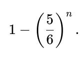
When r = 6, the probability that the largest roll is 6 is:

This makes intuitive sense because 1 − (5/6)^n is the probability that at least one roll turned out to be a 6.
Practical Implementation in Python
Here is a straightforward Python function to compute the probability that the largest number is r for each r in 1..6, given n:
def probability_largest_r(n, r):
    """Returns the probability that the largest face in n rolls is exactly r."""
    return (r/6)**n - ((r-1)/6)**n

# Example usage:
n = 5
for r in range(1, 7):
    print(r, probability_largest_r(n, r))
The function probability_largest_r(n, r) implements the exact formula. Notice that r must be between 1 and 6.
Potential Pitfalls and Considerations
It is critical to note that each roll is assumed to be independent and uniformly distributed over {1,2,3,4,5,6}. If the die were biased or if the rolls were not independent, the above formula would not hold. Additionally, floating-point imprecision can become significant when n is large, though in many practical settings for moderate n, double-precision floating-point arithmetic is more than sufficient.
If the problem were asked in a combinatorial format (like “in how many ways can the largest be r?”), you could derive the number of favorable outcomes as the difference between the number of ways all rolls can be from {1,...,r} minus the number of ways all rolls can be from {1,...,r−1}. That leads you to the same probability after dividing by the total number of outcomes 6^n.
Below are several deeper follow-up questions that commonly appear in interviews to probe the depth of your understanding, along with thorough explanations.
Suppose the interviewer asks: How can this approach be generalized if the die is not fair, meaning each face has a different probability?
If the die is not fair, then each face i (from 1 to 6) has some probability p_i with the constraint that p_1 + p_2 + p_3 + p_4 + p_5 + p_6 = 1. For the largest number to be r, we need all rolls to be in {1, 2, ..., r}, and at least one roll to be exactly r.
We can denote q(r) = p_1 + p_2 + ... + p_r as the cumulative probability of rolling a value at most r on a single trial. Then for n independent rolls, the probability that all outcomes are at most r is [q(r)]^n. Likewise, the probability that all outcomes are at most (r − 1) is [q(r−1)]^n. By the same logic of subtracting these probabilities, the largest is r with probability
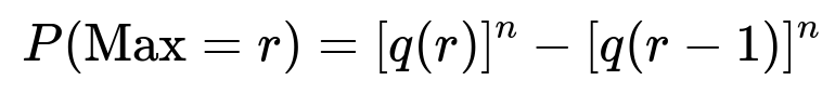
The only difference from the fair-die case is that q(r) is no longer r/6 but rather the sum of face probabilities up to r. Of course, one would need to know each p_i explicitly. The more general principle remains exactly the same: compute the probability that no roll is above r, then subtract the probability that no roll is above r − 1.
A tricky real-world issue with non-uniform distributions is ensuring that you correctly identify the probabilities p_i. In some practical scenarios (e.g., manufacturing defects in dice or special loaded dice), you might only have approximate estimates of these p_i. The formula then still applies with those estimates, but the reliability of the result depends on how well you have estimated p_i.
Suppose the interviewer asks: Could we arrive at the same formula using the Inclusion-Exclusion Principle?
Yes, though it can be a bit lengthier in logic. You can consider the event that “at least one die shows r.” Then you need to exclude cases where any die shows a value larger than r. Using Inclusion-Exclusion, you count the ways to get a maximum of at most r and then reason about exactly one or more dice being r. Ultimately, you would find that it leads to the same difference:

because Inclusion-Exclusion for “largest exactly r” is the complement of “largest ≤ r − 1” within “largest ≤ r.”
In some questions, you might see a more generalized Inclusion-Exclusion approach used to compute probabilities about the maximum or minimum values or about how many dice meet certain criteria. It is helpful to note that while Inclusion-Exclusion can always be used for these sorts of “at least/at most” events, the simpler direct approach we used is usually more elegant and efficient.
Suppose the interviewer asks: What if we want the probability that the largest number is at least some specific value k, where 1 ≤ k ≤ 6?
We can easily adjust. The probability that the largest number is at least k is the complement of the event that every roll is less than k. Every roll being less than k means all outcomes are from {1, 2, ..., k − 1}. So that probability would be

This is simply using the logic that “largest at least k” = “not (largest ≤ k − 1).”
Suppose the interviewer asks: Do we have to worry about floating-point precision for large n?
Yes, for very large n, expressions like (r/6)^n might become extremely small (potentially underflowing to 0.0 if n is huge) or extremely close to 1 if r is large relative to 6. In most practical data science or engineering settings, typical dice problems do not require n so large that standard double-precision arithmetic breaks down irreparably. However, if you were, say, generating a simulation of n in the range of billions or dealing with extremely small probabilities in a broad Monte Carlo analysis, you might want to consider using logarithms to keep track of the sums and differences more stably or use higher precision data types.
An example of using logarithms is to compute log probabilities:
If you wanted to compute

numerically, you could do
import math

log_prob = n * math.log(r / 6.0)
prob = math.exp(log_prob)
which is more numerically stable for large n compared to directly raising r/6 to the power n.
Suppose the interviewer asks: How can we verify the correctness of this formula experimentally?
One straightforward way is to run a Monte Carlo simulation. For instance, you can simulate a large number of experiments of n dice rolls, track the largest value from each experiment, and then compute the empirical frequency that the largest is r for r = 1..6. As the number of trials grows, the frequencies should converge to the theoretical probabilities.
Here is an example code snippet for verification:
import random
from collections import Counter

def simulate_largest_value(num_experiments, n):
    counts = Counter()
    for _ in range(num_experiments):
        rolls = [random.randint(1, 6) for __ in range(n)]
        max_val = max(rolls)
        counts[max_val] += 1
    for r in range(1, 7):
        print(r, counts[r] / num_experiments)

# Example usage:
simulate_largest_value(num_experiments=10_000_00, n=5)
Comparing the printed empirical probabilities with the closed-form solution will assure you that the formula matches real observations.
Suppose the interviewer asks: What if we want the distribution of both the largest value and the smallest value simultaneously?
That is a more detailed scenario. You would need to consider the probability that the smallest value is m and the largest value is r for some 1 ≤ m ≤ r ≤ 6. Then you would count the number of ways (or use the probabilities) such that all values lie in the set {m, m+1, ..., r} and that at least one value is m and at least one value is r. This can be done by an inclusion-exclusion approach or by subtracting out probabilities that do not meet the boundary conditions. The exact formula typically becomes more intricate:
All rolls must be in {m, m+1, ..., r} => Probability is ((r − m + 1)/6)^n Remove cases with no roll being m => Probability is ((r − m)/6)^n Remove cases with no roll being r => Probability is ((r − m)/6)^n Add back cases missing both m and r => Probability is ((r − m − 1)/6)^n
So the probability that the smallest is m and the largest is r becomes:

provided r ≥ m, which ensures there is at least one face in the set {m, ..., r}. That can be extended to more complicated simultaneous conditions on multiple dice statistics. The essential logic is always based on the difference of probabilities of being in certain subsets and not being in others.
Suppose the interviewer asks: Could there be a combinatorial expression that explicitly counts the number of favorable outcomes?
Yes, and it is totally equivalent. For the event “largest is exactly r,” we count how many outcomes have values only from {1, 2, ..., r}, which is r^n total ways, minus those outcomes that are only from {1, 2, ..., r-1}, which is (r−1)^n total ways. Each outcome has probability (1/6^n) in the fair-die scenario. Dividing by 6^n yields

which is exactly the same expression we have been working with. This method might be labeled the “counting approach” or “combinatorial approach,” whereas the approach we gave initially focuses more directly on probabilities. Both yield the same final answer.
Suppose the interviewer asks: Are there specific boundary conditions we can check to be sure the formula makes sense?
Check that the sum of probabilities over r = 1..6 is 1:
Each of these probabilities is also non-negative because (r/6)^n ≥ ((r − 1)/6)^n when r ≥ 1. Finally, for n = 1, we should get a uniform distribution for the largest value if we only roll once. Indeed, for n = 1:
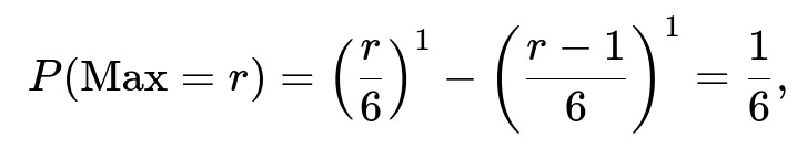
which is correct. Such checks confirm the internal consistency of the formula.
Suppose the interviewer asks: In a real-world scenario, how can we extend this to more than six-sided dice or to dice with custom faces?
All we really need is to define the set of possible faces. For a k-sided die with faces numbered 1..k, in the fair scenario, the probability that a single roll is at most x is x/k. Then for the largest to be exactly r:
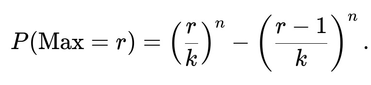
The entire logic is the same. We only swapped 6 for k in the fraction. For dice with custom-labeled faces, you first order them from smallest to largest and assign each face a position i in that sorted list. Then you adapt the same difference-of-cumulative-probabilities approach, using the distribution for a single roll to compute probabilities that the outcome is no larger than a particular face. The step from cumulative distribution to differences remains the same.
Below are additional follow-up questions
What if someone asks: “How do we derive or validate these probabilities if we only have partial outcome data, for instance, if some rolls are missing or censored?”
In certain real-world scenarios (or complicated data-collection experiments), you might not have a complete record of each individual roll. Perhaps some outcomes are missing, or you only know that the roll was at least a certain number but not exactly which. This situation can be understood through censored or missing data.
One way to address this is by applying techniques for missing data in probability and statistics:
• Maximum Likelihood Estimation (MLE) for incomplete data: You can write down the likelihood of the observed data (including partial or censored observations) using the known distribution for dice rolls, then optimize the parameters (like unknown bias parameters or even the quantity “largest is r”) to fit the partial observations. For a fair die with missing data, you can still rely on the assumption that each face has probability 1/6, but you might need to condition on the partial information for certain rolls. For example, if you know a certain roll was at least 3, you would treat that as a partial observation that excludes outcomes {1,2}.
• Bayesian approaches: You could also incorporate priors over the fairness or bias of the die and update your posterior beliefs based on partial data. For instance, if certain observations are only known to exceed 4, you update the likelihood accordingly.
Potential pitfalls or edge cases:
• If you have heavy censoring (e.g., most of the data is missing or you only know the roll outcome for a few trials), estimates of the probability “largest number is r” may be very uncertain. • If the underlying distribution is not truly fair, but you assume fairness, your final probability estimates can be significantly skewed. • Overfitting or underfitting can occur if you try to estimate more complicated die distributions from limited partial data.
What if the interviewer asks: “How can the distribution of the largest roll help us generate new random samples or perform tasks like data augmentation?”
When you know the distribution of the largest roll, it can guide how you simulate or augment synthetic data:
• Direct sampling approach: If you want to simulate a batch of n-roll outcomes where the largest roll is r with a certain probability, you can first decide which largest value you want for that simulation (using the probability formula), then sample the actual n outcomes constrained to that largest value. For example:
Choose r according to
Randomly assign which positions in your n-length sequence get the maximum r (at least one position must be r).
For the other positions, choose any integer from 1 to r (including the possibility of r for multiple positions, if you want the entire sample space consistent with “largest = r”).
• Data augmentation: In machine learning contexts, if your features or experiments revolve around dice outcomes, understanding the distribution of extreme values (like the max or min) can help you augment data to reflect certain probabilities of extremes. This might be relevant if you’re modeling game mechanics or random processes that revolve around “highest roll” events.
Potential pitfalls or edge cases:
• Constraining the largest value can bias the distribution of the other rolls if you are not careful in how you sample. For instance, once you fix the largest value as r, you must sample all other rolls uniformly from 1..r for a fair die, and ensure at least one is r. • If your end goal is to approximate the real distribution of all n-roll outcomes, you must preserve the correct fraction of times each r occurs as the maximum.
What if the interviewer asks: “Could the probability that the largest roll is r be used in hypothesis testing about the fairness of a die?”
Yes. If you suspect a die might be loaded, you could test the null hypothesis that the die is fair against alternative hypotheses that the die has a bias toward certain faces. You can:
Collect experimental data from multiple n-roll sequences.
Observe how often the maximum is 1, 2, 3, 4, 5, or 6 across many sequences.
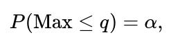
Compare this empirical distribution of the maximum with the theoretical distribution under the fair-die assumption:

Use a goodness-of-fit test like Pearson’s chi-square test to see if the observed frequencies differ significantly from the theoretical frequencies.
Potential pitfalls or edge cases:
• Sample size: If you do not roll the die enough times (or do not gather enough n-roll sequences), you might have insufficient statistical power to detect moderate biases. • Multiple comparisons: If you test many different die faces or multiple statistics (like the largest and smallest simultaneously), you should consider corrections for multiple hypothesis testing.
What if the interviewer asks: “How does the distribution of the largest roll change if each of the n dice has different possible faces? For example, one die is 6-sided and the other is 4-sided, etc.”
If you mix dice with different faces, the logic for “largest roll equals r” still involves:
• Defining the set of possible outcomes for each die and the probability distribution for each face. • Ensuring you consider only outcomes up to r for all dice, and subtract outcomes up to r−1 for all dice.
For instance, if you have two dice: • Die A is 6-sided (fair). • Die B is 4-sided (faces 1..4, fair).
Then the probability that the maximum is at most r depends on the combined distribution:
• If r ≤ 4, the probability that Die A ≤ r is r/6, and the probability that Die B ≤ r is r/4. So all dice at most r is (r/6)*(r/4). • If r > 4, you have to note that Die B can only go up to 4, so for r=5, for example:
Probability(Die A ≤ 5) = 5/6
Probability(Die B ≤ 5) = 1 (since Die B can only be 1..4).
Combined probability all dice ≤ 5 = (5/6)*1.
Once you generalize to n dice, each with potentially different face sets or different biases, you multiply all these single-die probabilities. Then to get “maximum = r,” you do:
Potential pitfalls or edge cases:
• If one die has fewer faces than r, it’s automatically always “less than or equal to r.” You must carefully handle these boundary conditions for each die. • Implementation details can get messy if you have many dice with different custom distributions. Good practice is to define a function that returns “probability(die_i ≤ x)” for each die i, then multiply them together.
What if the interviewer asks: “How does the probability that the largest is r factor into expected values or other summary statistics of the maximum?”
To compute the expected value of the maximum for a fair 6-sided die rolled n times, you can use:

Either way, the distribution of the maximum is central to computing such statistics.
Potential pitfalls or edge cases:
• For large n, the maximum tends to concentrate near 6, so the distribution becomes heavily skewed. Most of the probability mass eventually shifts to 6 as n grows large. • If you want higher moments (e.g., variance of the maximum), you can similarly use the distribution or relationships like

What if the interviewer asks: “In a real gambling game with multiple dice, might a ‘house edge’ approach relate to the probability that the largest number is r?”
Yes. If a game’s payout depends on whether a certain highest value is achieved, or if certain high rolls trigger bonus payouts, you can compute the expected payout by combining:
• The event probability (largest roll is at least some threshold, or exactly some value). • The payoff given that event occurs.
For instance, if the game pays $10 whenever the largest of n dice is 6, you compute:
• Probability of largest = 6:

You can generalize to multiple conditions (e.g., $5 if largest = 4 or 5, $10 if largest = 6, etc.) by summing over the probabilities of each condition times its payoff.
Potential pitfalls or edge cases:
• Non-mutually exclusive events with complicated bonus structures might require careful probability decomposition (e.g., if you get a partial bonus for having at least a 5, and an extra bonus for hitting 6, you need to break down the events or use Inclusion-Exclusion carefully). • Real gambling setups sometimes omit certain face values or alter the payouts to ensure a strong house edge. Make sure your assumptions about the die and game rules precisely match reality.
What if the interviewer asks: “How do these concepts extend to continuous variables or continuous distributions? For instance, if instead of rolling dice, we’re taking n samples from a continuous uniform distribution [0,1]. What is the probability that the maximum is less than or equal to some value x?”
Although not about discrete dice faces, the question is deeply related. For a continuous random variable X in [0,1], the probability that X ≤ x is simply x for x in [0,1], assuming a uniform distribution. For n i.i.d. samples, the event “all n samples ≤ x” has probability x^n. Thus, the event “maximum ≤ x” has probability x^n, leading to:
• Probability that the maximum is at most x:

• Probability that the maximum is exactly some value in a continuous sense is 0 at any precise point (since it’s continuous). Instead, we talk about the distribution function or the density function of the maximum. • The cumulative distribution function (CDF) for the maximum is

• The probability density function (PDF) for the maximum is the derivative:

Potential pitfalls or edge cases:
• In continuous settings, “probability that the maximum equals exactly r” (a single real number) is 0, so we must shift to the language of CDFs or PDFs. • Mixed distributions: If some portion of your sample space is continuous and some is discrete, you need to handle that carefully.
What if the interviewer asks: “How would you efficiently compute the probability distribution of the maximum if n is extremely large (like millions), where direct exponentiation might be computationally expensive or susceptible to floating-point underflow?”
For extremely large n, direct approaches like (r/6)^n can approach 0 or 1 too closely to be represented precisely in floating-point format. Here are strategies:
• Use log space arithmetic: Compute log((r/6)^n) = n ⋅ log(r/6). Subtract logs to get the difference in a stable manner (possibly using the “log-sum-exp” trick if you are dealing with a difference). • Use rational fraction approximations: Because (r/6)^n is rational, in principle you could store large exponents using symbolic libraries, though this is usually feasible only for moderate n. • Approximate expansions: For large n, (1 − α)^n can sometimes be approximated with

when α is small, or it might saturate near 1 if αn is large. This can be combined with bounding techniques to ensure numerical stability.
Potential pitfalls or edge cases:
• Rounding errors might accumulate if you do naive exponentiation or repeated multiplication. • Subtraction of nearly equal quantities (like 1 − (5/6)^n) can cause catastrophic cancellation if (5/6)^n is close to 1. Using log space or stable expansions is the safer approach.
What if the interviewer asks: “How does the probability that the largest is r connect to the median of the maximum or other quantiles?”
The distribution of the maximum can be used to find any quantile of the maximum. For instance, the median is the point m such that:

In the discrete die scenario, you would solve for the smallest integer m that satisfies:
In other words, you check cumulatively from m = 1 upward until
Then m is the median. More generally, for a continuous distribution or for a loaded die, you solve for m using the known cumulative distribution of the maximum. This approach extends to other quantiles (like the 90th percentile, etc.):
where α might be 0.9 for the 90th percentile. Solve for q accordingly.
Potential pitfalls or edge cases:
• For discrete distributions, the quantile might not be uniquely defined if the distribution jumps at certain points. • For large n, the median of the maximum for a fair die will quickly move toward 6 because half the time you see at least one 6 if n is large enough. You might find the median to be 6 after n reaches a certain threshold.
What if the interviewer asks: “How can knowledge of the maximum distribution help in analyzing sums or other statistics of dice?”
Sometimes, you might not only want the maximum, but also the sum of the dice. The distribution of the maximum and the sum are related but are not independent. For example, if you know the maximum is small, that constrains the sum to be relatively small as well. While the sum of n fair dice is well-known to follow a discrete convolution of uniform distributions (often approximated by a normal distribution for large n via the Central Limit Theorem), the maximum can help refine your analysis. For instance, if the maximum is 6, that might push the sum distribution’s tail upward relative to the scenario of “maximum ≤ 5.”
Potential pitfalls or edge cases:
• Summaries like “average roll” or “sum of the dice” do not factor neatly with “maximum.” They have complex dependencies. • If you want joint distributions (like “the sum is S and the maximum is r”), you might need more sophisticated counting or dynamic programming to account for all possible combinations of n dice. • If the dice are not fair, each distribution changes in a way that must be handled carefully.
What if the interviewer asks: “Could we interpret the maximum roll as a random variable in the context of order statistics, and how does that relate to minimum or median rolls?”
Yes. In probability theory, the maximum of n i.i.d. samples is the nth order statistic. If you label the rolls X₁, X₂, ..., Xₙ, sorted from smallest to largest as X_(1) ≤ X_(2) ≤ ... ≤ X_(n), then X_(n) is the maximum. Similarly, X_(1) is the minimum, X_(k) is the k-th smallest, and so on. Standard formulas exist for the distribution of these order statistics in both discrete and continuous cases. For a fair die:
• X_(n) = max(X₁, ..., Xₙ). • X_(1) = min(X₁, ..., Xₙ).
In general, for continuous distributions, the PDF of X_(k) is given by a Beta function-related expression. For discrete dice, you can count ways to achieve a particular ordering pattern.
Potential pitfalls or edge cases:
• The more complicated the statistic (like the 2nd largest or the median), the more intricate the counting or inclusion-exclusion can become in discrete cases. • Real-world measurements might have ties or other non-ideal phenomena (like repeated values in continuous distributions or sensor noise), requiring careful adaptation of the standard order statistics approach.
What if the interviewer asks: “How might real-world dice exhibit correlations between rolls (e.g., if the die is physically damaged and tends to roll certain faces more often in certain sequences), and how does that affect the maximum distribution?”
If the rolls are not strictly independent, the entire derivation for “P(Max = r)” no longer holds in its original form. The formula
assumes each roll is an independent event from a distribution that is the same for each roll (i.i.d.). If there are correlations—e.g., the outcome of one roll influences the next—then:
• You cannot just multiply the single-roll probabilities. • You must model the joint probability distribution of (X₁, X₂, ..., Xₙ). • The event “maximum ≤ r” becomes the event “all Xᵢ ≤ r.” You would need to integrate (or sum) over the joint distribution for all i.
For a physically damaged die that biases certain faces in a correlated manner from roll to roll, you would need to:
• Empirically measure or estimate the transition probabilities from one outcome to the next. • Possibly build a Markov chain or a more complex dependency model. • Derive or simulate the distribution of the maximum from that model.
Potential pitfalls or edge cases:
• Overlooking even slight correlation can skew the distribution of extremes if certain “streaks” of high or low rolls are more likely. • In real dice, correlations might be negligible if the die is well-shaken between rolls. In partial or lazy rolling (e.g., the die is only lightly flicked), correlations might be more substantial.
What if the interviewer asks: “For a large number of dice, how quickly does the probability that the maximum is 6 approach 1? Is there a threshold where it becomes almost certain?”
For a fair 6-sided die rolled n times, the probability that the maximum is 6 is:

As n grows large, (5/6)^n shrinks exponentially toward 0, so the probability of seeing at least one 6 quickly approaches 1. Specifically, if (5/6)^n < 0.01, that means there is at least a 99% chance the maximum is 6. Solving:

In practice, for n ≈ 15 to 20, you already see a pretty high probability of getting at least one 6. After about 20–25 rolls, it becomes extremely likely that 6 appears at least once.
Potential pitfalls or edge cases:
• For a biased die that heavily disfavors 6, even large n might not guarantee the maximum is 6 with high probability. • For a different number of faces or partially known distributions, you need to re-apply the same logic but with the appropriate parameter for “probability of not rolling that highest face.”
What if the interviewer asks: “How would these probabilities change if after rolling the die n times, we remove the lowest roll (or some subset of rolls) and only keep the rest, then define the maximum over the subset?”
Once you remove certain rolls from the set, the distribution of the “maximum of the remaining rolls” changes. For instance, if you always discard the smallest single roll among n, you effectively keep n-1 rolls. But these n-1 rolls are not quite i.i.d. from the original distribution because they are specifically “all but the minimum.” This selection condition means the distribution of retained dice is not the same as the distribution of all dice rolled independently.
An exact approach:
Consider the random vector of n i.i.d. dice outcomes.
Identify which outcome is the minimum (ties require more careful counting).
Discard it.
The maximum of the remaining n-1 depends on the entire joint distribution plus the tie scenarios.
You can do direct counting for small n, but the formula gets complicated. Another approach is to simulate:
• Generate many n-roll outcomes, remove the lowest roll, track the maximum among the remaining, and approximate the probability distribution.
Potential pitfalls or edge cases:
• Ties in the minimum can complicate which roll you are removing (e.g., if there are two or more occurrences of the minimum value). • If the question arises from a real gaming rule (e.g., “roll four six-sided dice, drop the lowest one, sum the rest”), be sure to incorporate exactly how the game handles ties or reorderings.

Potential pitfalls or edge cases:
• If r=1, then Bᵣ = B₁ is the event that all dice ≤ 0, which has probability 0. This must be handled carefully in code to avoid negative indices or nonsensical probabilities. • Make sure r≥1 is valid. If you tried to compute P(Max = 0) or P(Max = 7), that is outside the space of normal dice values and can lead to errors if not accounted for in code.
What if the interviewer asks: “How do we incorporate the concept of the largest roll into a Markov Decision Process (MDP) or Reinforcement Learning framework, for example in board game simulations?”
In some game scenarios (like certain dice-based board games), decisions can depend on whether the largest roll meets a threshold. You could define:
• State: The partial sequence of rolls so far, or the number of rolls left, plus knowledge of the largest value observed so far. • Action: The choice to continue rolling or to stop, or any other strategic decision. • Transition probabilities: The probabilities of rolling each possible face on the next roll. • Reward: Possibly a function of the largest roll (e.g., a bonus if you eventually reach at least a 5 or 6).
When modeling this in an MDP, “largest so far = r” might be part of the state dimension. Then, at each step, you compute how that state transitions to “largest so far = max(r, new_roll).”
Potential pitfalls or edge cases:
• State space explosion: If you track the largest roll so far, that adds to the dimensionality of the state. For many dice or a large number of possible outcomes, the state space becomes huge. • Approximations or function approximators might be needed to handle large or continuous action spaces. • If the die is biased or has memory, then the transition is not simply “largest so far, r → largest so far, max(r, new_roll) with probability p(new_roll).” You must incorporate the correlation structure in how the die transitions from one roll to the next.
What if the interviewer asks: “Is there a connection between the maximum of n dice and the coupon collector’s problem, or other collecting/bingo problems?”
While they are not exactly the same phenomenon, there is a thematic link: the coupon collector’s problem is about how many draws you need to collect each of multiple coupon types at least once. By contrast, “largest is r” is about whether at least one instance of face r (or higher) appears. In coupon collector, you want at least one occurrence of each face from 1..6; in the largest face problem, you only require at least one occurrence of face r or above.
However, you can see some structural similarities:
• Both problems rely on the idea of “at least one success in a set of trials.” • They differ in that coupon collector typically wants every face to appear (a more stringent condition), whereas the maximum roll being r is a simpler condition of whether or not certain faces appear. • In coupon collector, the distribution of the time to collect all faces is tricky and typically leads to harmonic numbers. For the maximum, it’s a simpler expression because it’s a single threshold event rather than multiple events all needing to happen.
Potential pitfalls or edge cases:
• If a question tries to conflate the two, be careful. They have distinct probability structures. • Some interview questions might be “trick” questions that reference coupon collector logic but then ask about maximum; clarifying the difference is important.
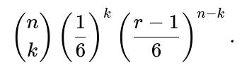
What if the interviewer asks: “Could we combine the probability of the largest roll with the distribution of how many times that largest roll appears? For instance, what is the probability that the largest roll is r and it appears exactly k times among the n dice?”
Yes. This becomes a more granular distribution question. If the largest roll is r, we want exactly k dice that landed on r, and the other n−k dice are all ≤ r but not equal to any number greater than r. More precisely:

for each of those n−k dice).
But we must combine this logic carefully with the fact that no dice exceed r. • A simpler approach is to consider the distribution of all dice from {1, 2, ..., r} and at least one r. Then among that scenario, count the fraction that have exactly k occurrences of r.
One direct combinatorial approach:
Probability that a single roll is in {1, ..., r−1} is

and the probability that it is exactly r is

Probability that exactly k out of n are r, and the others are at most r−1, is:

But that set includes the possibility that the other n−k dice could be less than r but not necessarily restricting the maximum among those n−k to be less than r. Actually, that’s okay if we interpret “largest is r” as “the other dice are at most r, and at least one is exactly r.”
Sum over k=1..n (since we need at least one r). Or if you want exactly k occurrences of r, pick that specific k.


Potential pitfalls or edge cases:
• Double counting or missing the event that the maximum might actually be bigger than r if you do not handle the bounding logic properly. • Implementation details can get tricky; verifying with direct combinatorial arguments or simulation can help ensure correctness.
What if the interviewer asks: “How can we apply these ideas about the largest roll in a scenario where n is random itself? For instance, we roll a die repeatedly until we get a 1 or we exceed some threshold of sum, and then we ask about the distribution of the largest roll in that process?”
This is a stopping time scenario, where n is not fixed but is itself a random variable. The distribution of the largest roll is then a mixture over the different possible values of n:
• We define a random variable N that depends on some stopping rule. For each possible n, there is a probability that we stop exactly at n. • Conditional on stopping at n, the distribution of the maximum is the same as the standard “largest of n dice.” • So the unconditional distribution of the maximum is:

Of course, in practice, N might have a distribution that eventually ensures we stop. You then combine that distribution with

Potential pitfalls or edge cases:
• The sum might not converge to an infinite series if the stopping condition is complicated; you need to carefully define P(N = n). • Markov chain or state-based modeling is often used if the stopping rule depends on the sum or on seeing a particular face. Then you might handle the distribution of the maximum by enumerating all possible states or using simulation.
What if the interviewer asks: “In a large simulation codebase, how do we ensure we handle the floating-point computations for probabilities like (r/6)^n consistently across languages (e.g., Python vs C++ vs Java)?”
Implementation details often cause small numeric differences in computed probabilities. Key best practices include:
• Using double precision (float64 in Python) rather than single precision wherever possible. • Employing the math library’s functions (like math.pow, math.log, etc.) carefully. • Being consistent with how you structure computations. For instance, if you do repeated multiplication in a loop, you might accumulate floating-point errors differently compared to a single call to pow() or exp(n * log(x)).
Potential pitfalls or edge cases:
• If n is huge, even double precision might underflow (leading to 0.0). • If your code runs on a GPU (e.g., with PyTorch), watch for half precision vs single vs double. This can drastically affect the stability of the result. • When probabilities approach 1 or 0, direct subtraction “1 - x” can lose precision if x is extremely close to 1 (catastrophic cancellation). A typical approach is to keep track of log(1−(5/6)^n) via a log-sum-exp trick or use expansions for small x.
What if the interviewer asks: “How would you adapt your answer if we define the ‘largest number rolled’ in a special sense, like ignoring or re-rolling certain outcomes?”
In many tabletop or gaming house rules, you might see instructions like, “Roll a die, but if you get a 1, you re-roll once. Take the largest number you see from all attempts.” That modifies the distribution of each individual attempt:
The single-roll distribution is no longer uniform; you have a second chance if the first roll is 1. This changes the probability that the final outcome (the effective single-roll value) is each r in {1..6}.
Once you define the distribution for a single “effective roll,” then for n “effective rolls,” you can apply the same maximum logic. But first, you must carefully derive

For example, ignoring 1 and re-rolling:
• Probability of effectively rolling a 1 might become (1/6)*(1/6) = 1/36 if you keep re-rolling after the first is 1 but get 1 again. • Probability of effectively rolling 2..6 must be recalculated accordingly.
After each single “effective roll” distribution is known, your usual maximum formula

will handle the event that all n “effective rolls” are at most r, minus all at most r−1.
Potential pitfalls or edge cases:
• If re-rolls can cascade or if there is a limit to re-roll attempts, the single-roll distribution might be even more complicated. • Make sure to handle tie events or partial ignoring rules (e.g., “ignore the first 1, but if you roll 1 again on the re-roll, keep it”). Each variation changes the distribution.
What if the interviewer asks: “In a game theory setting, if multiple players each roll n dice, what is the probability that a particular player ends up with a strictly larger maximum than all other players?”
If each player i rolls n dice, we define Mᵢ as the maximum result of that player’s n dice. The question becomes:

for k players total. • Assuming all dice across all players are fair and independent, you can approach this by computing the distribution of M_1, M_2, …, M_k and sum over the event that M_1 is strictly greater than each M_j for j=2..k.
One direct method:
Probability that M_1 = r is
Probability that each other M_j ≤ r−1 is

So, you could sum from r=1..6:

This counts the scenario where M_1 = r and each other M_j is at most r−1.
Potential pitfalls or edge cases:
• Handling ties: If you want a strictly larger maximum, you exclude cases where M_j = M_1. If you want the probability that player 1 is at least tied for the largest, you include those equal cases. • For large k, the probability that everyone else has a maximum ≤ r−1 can be quite small for high r. • Implementation detail: Summations or exponentiations might be large or small, requiring stable numeric methods.
What if the interviewer asks: “How do we handle multiple ‘largest values’ conditions at once, like the probability that the largest is exactly 4 or 6, ignoring the possibility of 5, or that the largest is in the set {2, 4, 6}?”
If you want the probability that the largest is in a certain subset S of {1,2,3,4,5,6}, you can sum up:

But if you specifically want the maximum to be either 4 or 6—meaning it cannot be 5, and it cannot exceed 6—then:

trivially for a standard 6-sided die. •

But if you need an approach that excludes 5 from the set of possible maxima, you must be sure to not double-count or incorrectly include the scenario “maximum=5.” The difference-of-cumulative approach is straightforward:

Summing the appropriate terms gives the event that the max is exactly 4 or exactly 6.
Potential pitfalls or edge cases:
• If S is large, you might prefer 1 minus the probability that the max is in the complement set. • For real code, enumerating sets or subsets can be done carefully with sums of the basic “max=r” probabilities.
What if the interviewer asks: “How do you interpret the event that the largest number rolled is r if the dice are not all 6-sided but some have more sides than 6?”
If at least one die has more faces (say a 10-sided die with faces 1..10), the largest possible outcome can exceed 6. Then the event “largest is exactly r” with r ≤ 6 must incorporate that the 10-sided die did not show any face bigger than r. If r is smaller than the maximum face of that die, you have to multiply in the probability that the 10-sided die’s result is at most r.
If r is smaller than the number of faces for multiple dice, you combine each die’s “≤ r” probability. Then subtract the probability that all dice are ≤ r−1:
[∏i=1kP(die i≤r)]−[∏i=1kP(die i≤r−1)].

Potential pitfalls or edge cases:
• If a die’s maximum face count is less than r (for example, you have a 4-sided die and r=5), you need to treat the probability “die ≤ 5” as 1 for that die. • If you have a weird distribution or partial knowledge about the custom dice, you need an accurate model for each die’s probability distribution up to r.
What if the interviewer asks: “How can we check that, across r=1..6, the probabilities for the largest roll sum to 1 in code, and what might cause them not to sum exactly to 1 in floating-point arithmetic?”
To verify:
import math

n = 10
sum_p = 0.0
for r in range(1,7):
    p = (r/6)**n - ((r-1)/6)**n
    sum_p += p

print(sum_p)  # Should be very close to 1.0
You might see something like 0.9999999998 or 1.0000000002, etc., because floating-point arithmetic introduces rounding. That discrepancy is typically on the order of machine epsilon, around 1e-15 in double precision.
Potential pitfalls or edge cases:
• If you see a large discrepancy (like 0.95 or 1.05) for moderate n, that suggests you made a coding or logic error (typo, indexing issue, etc.). • For very large n (thousands or millions), one or more terms might underflow to 0.0, or you might get (r/6)^n = 1.0 if r/6 is extremely close to 1. • In those cases, using log domain or carefully rearranging computations is recommended.
What if the interviewer asks: “How might we handle symbolic mathematics software (like Sympy in Python) to do an exact combinatorial check for these probabilities?”
In symbolic math packages, you can write:
import sympy as sp

r, n = sp.symbols('r n', positive=True)
expr = (r/sp.Integer(6))**n - ((r-sp.Integer(1))/sp.Integer(6))**n
Then you can perform expansions or simplifications symbolically. For instance, for r=6:
expr_simplified = sp.simplify(expr.subs(r, 6))
print(expr_simplified)
It should simplify to
Potential pitfalls or edge cases:
• Symbolic expressions can get large or complicated if you do expansions of (r/6)^n for general n. • If you want integer expansions (like r^n), that might create large polynomials for symbolic expansions. • For large n, purely symbolic expansions can be slow or memory-intensive.
What if the interviewer asks: “What if the dice are labeled differently, like a standard ‘Sicherman dice’ arrangement or any custom-labeled dice that still produce certain sums, does the maximum roll formula remain the same?”
Sicherman dice are a special pair of dice that yield the same sum distribution as two standard 6-sided dice but with different face labels. Even though the sum distribution matches, the largest face distribution will differ because the label arrangement is not standard.
The standard formula “largest is exactly r” relies on each face from 1..6 appearing with probability 1/6 on a single standard fair die. If your die is labeled with non-sequential or repeated numbers, you must define:
• Probability that a single die’s outcome is ≤ r. • Probability that it is ≤ r−1.
Then for n dice, multiply those probabilities. So the logic “(r/6)^n - ((r-1)/6)^n” no longer directly applies because “r/6” is only correct if the probability that a single die ≤ r is r/6. If the faces are labeled in unusual ways, you re-calculate that distribution. For Sicherman dice specifically, you might have a label set like {1,3,5,6,8,10} on one die, etc. Then you check how many of those labels are ≤ r for each die.
Potential pitfalls or edge cases:
• Don’t assume standard labeling means standard distribution for the maximum. They might preserve certain sum properties but differ drastically in maximum or minimum distributions. • Real usage might require enumerating or storing the face labels in a list and counting how many are ≤ r, then dividing by the total number of faces.
What if the interviewer asks: “Can these ideas about the largest roll be used in advanced ML tasks, such as analyzing the maximum activation in a neural network layer?”
Yes. In deep learning, the concept of “max pooling” or “maximum activation” can be conceptually related to the distribution of maximum values among a set of neurons. For instance, if each neuron’s activation is considered a random variable with some distribution, then the maximum across a patch is:

assuming independence. In practice, neuronal activations are not strictly independent nor identically distributed, so the formula is only approximate. Still, the analogy remains: the maximum of multiple random variables is simpler to handle if they are identically distributed and independent.
Potential pitfalls or edge cases:
• Neuronal activations typically have correlations. That means you can’t factor the distribution of the maximum into a simple product of marginals. • Activation distributions might be heavy-tailed (e.g., ReLU layers) or truncated (if you do clipping), so you might need specialized modeling if the distribution of the maximum is crucial.
What if the interviewer asks: “Is there a direct combinatorial formula for P(Max ≤ r) without relying on exponentiation?”
Yes. Counting approach for a fair 6-sided die:
• The total number of equally likely outcomes for n rolls is 6^n. • For Max ≤ r, all n rolls must come from the set {1,2,...,r}, which yields r^n equally likely outcomes out of 6^n. • So P(Max ≤ r) = r^n / 6^n = (r/6)^n. • Then P(Max = r) = (r^n - (r-1)^n)/6^n, which is the same as

You could do the same for the event Max = r by enumerating outcomes from {1,..,r} minus outcomes from {1,..,r-1}, that is r^n − (r−1)^n. Then dividing by 6^n. This direct count is typically how teachers first introduce the concept in combinatorics.
Potential pitfalls or edge cases:
• If r=6, (r−1)^n = 5^n. The difference 6^n−5^n must be computed carefully for large n to avoid overflow in integer arithmetic in some languages. • For partial knowledge or biased dice, the direct combinatorial approach is replaced by summing probabilities for each face, rather than counting uniform outcomes.
What if the interviewer asks: “How do we interpret the probability that the largest roll is r if we physically combine multiple dice into a single throw? For example, rolling n dice physically together vs. rolling them one at a time. Does that matter?”
Mathematically, as long as each die is distinct but identically distributed, rolling them all at once is still the same as rolling them sequentially. Probability theory does not distinguish between the order or simultaneity of the rolls. Each die remains an i.i.d. random variable with uniform distribution from 1..6. So:
• The distribution of the maximum is unchanged whether you physically throw them all at once or throw them in separate intervals. • Similarly, if you do partial re-rolls or anything else that changes the independence assumption, that must be accounted for, but standard simultaneous rolling does not alter the distribution.
Potential pitfalls or edge cases:
• Real-world friction or collisions among dice could introduce minuscule correlations in physical outcomes, but typically this is negligible for well-separated dice. • If you roll dice in stages and only keep certain dice (like in the game Yahtzee), that modifies the sample space from one stage to the next. Then the formula for the final maximum is more complicated.
What if the interviewer asks: “Why might the difference-of-cumulative approach be the best conceptual approach for ‘largest = r,’ rather than trying to count or sum more complicated events?”
The difference-of-cumulative approach is concise because of this nesting property:
• “Max ≤ r” is simpler to handle, as it does not require you to track how many dice show r or anything else, just that no die exceeds r. • Once you know “Max ≤ r,” you immediately have “Max ≤ r−1” as a strict subset. The difference between these two events is precisely “Max = r.” • It avoids the complexity of enumerating exactly how many dice show the value r, r−1, etc., or using Inclusion-Exclusion for each face above r.
Hence, from a conceptual standpoint, it is the most direct route to the final probability formula. It also scales well to situations where you have multiple categories for the random variable.
Potential pitfalls or edge cases:
• Make sure r is in a valid range. If r < 1 or r > 6, the formula might become nonsensical without special handling. • If the distribution is not i.i.d., the difference-of-cumulative approach must be replaced by more general arguments (though you can still do “P(all ≤ r) − P(all ≤ r−1)” for the joint distribution, just not factorized as in the i.i.d. case).
What if the interviewer asks: “How do you personally, as an expert engineer, debug or confirm your formula in a complicated scenario where the maximum’s distribution is not obviously known?”
Debugging typically proceeds through multiple steps:
Start with a small number of dice (e.g., n=2 or n=3) for which you can manually list out all possible outcomes or do a small script to generate them exhaustively. This ensures you can compare your theoretical formula to a brute-force enumeration.
Once you confirm correctness for small n, scale up to larger n with Monte Carlo simulation. Compare the empirical frequencies from the simulation to your theoretical result. They should match within random sampling error.
Use consistency checks: ensure that the sum of probabilities over r=1..6 is 1, check boundary cases (n=1, n=0 if that makes sense, r=1, r=6, etc.).
If you see discrepancies, look for off-by-one errors in the exponent, or index errors in how you handle the range of faces.
Potential pitfalls or edge cases:
• If the dice have custom probabilities or the scenario has partial or correlated data, you cannot do a direct enumeration easily. You might rely more heavily on simulation. • Very large n can cause numeric issues, so testing moderate n helps confirm the correctness before tackling the large-n regime.


