
ML Interview Q Series: Maximum Likelihood Estimation for Uniform Distribution Bounds

Browse all the Probability Interview Questions here.
7. Say you draw n samples from a uniform distribution U(a, b). What is the MLE estimate of a and b?
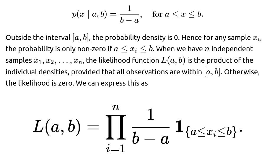
Understanding Maximum Likelihood Estimation (MLE) for the Uniform distribution can be very intuitive if we look at the geometry of the problem. However, let’s delve into the details, step by step, to give the strongest possible reasoning. We want to consider the distribution:

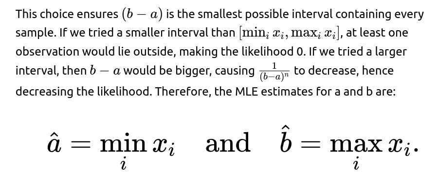
This result aligns perfectly with intuition: to fit a uniform distribution via MLE, you essentially want to pick the smallest observed value as the estimated lower bound and the largest observed value as the estimated upper bound.
A deeper explanation behind why these are indeed the MLE solutions is that any deviation from these extremes would either (1) exclude some sample points from the domain of the uniform or (2) unnecessarily expand the interval, reducing the height of the uniform density and hence lowering the likelihood. The MLE solution precisely “pins” the edges of the distribution to the outermost data points.

You can also see how easily this can be coded in Python if we assume your samples are in a NumPy array called “samples”:
import numpy as np

def uniform_mle_params(samples):
    a_hat = np.min(samples)
    b_hat = np.max(samples)
    return a_hat, b_hat

data = np.array([1.2, 2.5, 3.7, 2.9, 1.8])
a_est, b_est = uniform_mle_params(data)
print("MLE estimate for a:", a_est)
print("MLE estimate for b:", b_est)
This code snippet reflects the idea: estimate a by the minimum of the sample data, and estimate b by the maximum.

What if the data is not truly uniform in real-world scenarios?
In many real-world applications, data might approximate a uniform distribution but not match it perfectly. The MLE procedure remains the same: you find the smallest and largest data points as your best estimate for the bounds. However, in practice, you might want to consider outliers. A single outlier might greatly shift your a or b estimates, creating a very large interval and lowering the overall density. This can be problematic if the distribution is only “near-uniform” or truncated in reality. Practitioners might resort to robust methods or consult domain knowledge to decide if some extreme values should be removed or if a Bayesian prior should be considered.
How do outliers affect the MLE estimate for U(a, b)?
The uniform distribution by its mathematical definition requires that the entire range is captured. So a single outlier that is extremely large (or small) extends your uniform range drastically, resulting in a wide interval. This phenomenon can cause a wide uniform distribution with a small height (since 1/(b−a) becomes smaller if b−a is large). If you truly believe the data is uniform with no reason to discard that outlier, the MLE approach forcibly includes that outlier in the domain, producing the correct (though perhaps undesirable) estimate. In practice, if you suspect that outliers may come from measurement error or from a different data-generating process, you might adopt a more nuanced approach, possibly a robust variant or a truncated outlier removal approach.
Could we do a Bayesian approach for a and b?

How can we verify the MLE solution is indeed optimal?

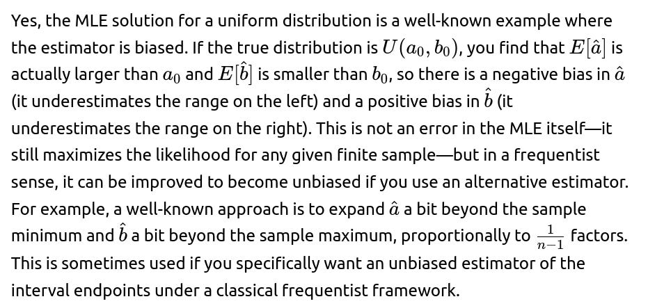
Could there be a bias or an alternative solution?
Potential pitfalls in implementing the uniform MLE approach in code
One pitfall is the presence of any data point that is unexpected or incorrectly measured. Because the uniform distribution is extremely sensitive to outliers (the largest or smallest point dominates the estimate of the entire range), even a single measurement error or outlier can cause the interval to become very large. In real-world data pipelines, it’s common to run outlier detection or sanity checks prior to committing to a uniform distribution assumption. Another pitfall is if the distribution is not truly uniform. Sometimes you might approximate something with a uniform distribution for convenience, but the data might be heavily skewed or follow a different shape. The MLE method described above will produce correct estimates for a pure uniform distribution, but it might perform poorly if your assumption is severely violated.
Conclusion of the MLE for a uniform distribution
Based on the likelihood analysis, the MLE solution to find the parameters of the uniform distribution U(a,b) is simply:
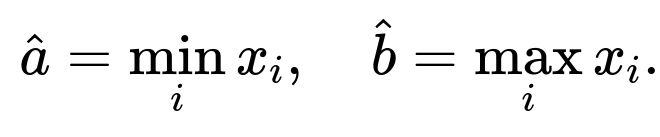
This result follows from the fact that you must include all samples in the interval for a non-zero likelihood, and shrinking the interval to exactly the range of the data points maximizes the likelihood. All deeper considerations—outliers, bias, Bayesian approaches—do not change this fundamental MLE result, but they do come into play in practical scenarios where data may not be perfectly uniform or might contain anomalies.
Below are additional follow-up questions
Suppose we had a situation where we only observe data points in a specific sub-range of the true uniform distribution. How does that affect the MLE estimates for a and b?


How do floating-point precision issues in real implementations influence the MLE for a and b?

What if the data comes from a uniform distribution on a circle or some other bounded manifold? Does the MLE for a, b still apply?

Can the MLE estimation fail if there is a known gap in the data?

In practice, encountering a big empty gap strongly suggests the data might not be drawn from a single U(a,b). A common remedy is to check for multi-modal behavior. If discovered, you might consider a mixture of uniform distributions or conclude that the uniform assumption is violated. The MLE formula for a single uniform distribution won’t fail mathematically, but it may fail as a model of reality.
What if the data’s true distribution is uniform but it has discrete rounding to certain intervals—like integers only? Does the continuous uniform MLE differ from a discrete uniform MLE?

In real tasks, if the data is only roughly discrete or the data frequency is extremely high, the difference between a continuous vs. discrete uniform might be negligible. But if you have small integer support (like {1,2,3,4,5}), the difference can matter. You can test goodness-of-fit or compare how well each approach captures the distribution.
What if we fit a uniform distribution in an online fashion—i.e., streaming data arrives one point at a time?

How do we handle negative values for a and b if the data is centered around negative or zero ranges?

Is there a closed-form expression for the variance of the MLE estimators a-hat and b-hat?

Could we apply a transformation to the data before applying the MLE for a and b?

What if the sample size is extremely small—like n=2 or n=3? Is MLE still reliable?

How would the MLE approach be adapted if we know that a must be non-negative, or if b cannot exceed a certain known value?

How do we incorporate repeated data points or weighted observations?

Can we use likelihood ratio tests or confidence intervals for the uniform distribution boundaries?

If you are in a role where precise error bounds matter—like bounding reliability or worst-case performance—understanding how to build confidence intervals from the uniform MLE is crucial. For large samples, standard approximations can be used. For small samples, exact or near-exact methods via order statistics are typically employed.