ML Interview Q Series: Maximum Likelihood Estimation for Exponential Rate λ in Lifetime Modeling

Browse all the Probability Interview Questions here.

14. Say you model the lifetime for a set of customers using an exponential distribution with parameter λ, and you have the lifetime history of n customers. What is the MLE for λ?

Understanding the exponential distribution and its maximum likelihood estimator is a crucial part of many machine learning or statistical modeling scenarios. The exponential distribution is commonly used to model time-to-event data or lifetimes, particularly because of its memoryless property and simplicity. Below is a thorough explanation of how to derive the MLE for λ, details on how to interpret it, considerations for edge cases, and follow-up question explorations.

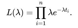
Log-Likelihood and MLE Derivation for λ Suppose we have n independent observations of customer lifetimes: t₁, t₂, …, tₙ. We assume each Tᵢ follows the same exponential distribution with parameter λ. We want to find the value of λ that maximizes the likelihood function. The likelihood L(λ) is the product of the individual PDFs evaluated at each observed lifetime:

To make it more convenient, we generally take the natural logarithm of the likelihood. This log-likelihood is:

ln(L(λ)) = ln(λⁿ) - λ ∑(tᵢ).

Because ln(λⁿ) = n ln(λ), the expression becomes:

ln(L(λ)) = n ln(λ) - λ ∑(tᵢ).

We want to find the λ that maximizes ln(L(λ)). To do so, we differentiate with respect to λ and set it to zero:

∂/∂λ [ n ln(λ) - λ ∑(tᵢ) ] = (n / λ) - ∑(tᵢ) = 0.

Rearranging gives:

n / λ = ∑(tᵢ).

Thus,

λ = n / ∑(tᵢ).

To confirm that this critical point is indeed a maximum, we can check the second derivative or use standard knowledge of exponential families. The second derivative is negative at that point, which indicates a maximum. Hence, the maximum likelihood estimator for λ, denoted λ̂, is:

This expression tells us that the estimated rate parameter is the reciprocal of the sample mean lifetime. Intuitively, if you have n independent observed lifetimes t₁, t₂, …, tₙ, and their average is (1/n) ∑(tᵢ), then λ̂ is 1 over that average.

Practical Examples of Computing the MLE in Python Below is a simple Python snippet showing how one could compute λ̂ given a list (or NumPy array) of observed lifetimes:

import numpy as np

def mle_exponential(data):
    # data is a list or numpy array of lifetimes t_i
    # MLE for λ is n / sum of t_i
    n = len(data)
    total_lifetime = np.sum(data)
    lambda_mle = n / total_lifetime
    return lambda_mle

# Example usage:
observed_lifetimes = [2.3, 1.9, 3.2, 4.1, 2.0]
lambda_estimate = mle_exponential(observed_lifetimes)
print("Estimated λ:", lambda_estimate)

In real-world settings, you might use a library function (e.g., in scipy.stats) to fit distributions, but under the hood, this is effectively what it does for the exponential distribution.

Interpretation of the MLE If we interpret Tᵢ as the lifetime or time-to-event, then λ̂ = n / (∑tᵢ) can be interpreted in two ways: • It is the rate parameter of the exponential distribution that best fits the observed data in the likelihood sense. • The mean lifetime is then 1 / λ̂ = (∑tᵢ) / n, which is just the sample mean. Because the exponential distribution’s theoretical mean is 1 / λ, the estimator for the mean lifetime is consistent with the sample average.

Memoryless Property Reminder The exponential distribution is memoryless, meaning P(T > s + t | T > s) = P(T > t). This property can be useful in certain modeling contexts (like queueing or reliability analysis). However, it also implies that if the data do not exhibit a memoryless type of behavior, the exponential model might not fit well. Nevertheless, if the exponential distribution is indeed appropriate, then the MLE formula above is straightforward.

Potential Issues in Real-World Data In practice, one must be aware that data might have: • Censoring (some customers may still be “active” at the time of data collection, so the total lifetime is not fully observed). • Reliability concerns (if the exponential assumption does not hold, or lifetimes have a heavier tail, a more general distribution such as Weibull might be more suitable). • Extreme values or measurement errors.

Despite these practical scenarios, if we assume fully observed lifetimes from an exponential distribution, the MLE formula above is exact.

Follow-up Question 1: Why do we use the log-likelihood instead of directly maximizing the likelihood?

We use the log-likelihood for mathematical and computational convenience. The likelihood is the product of individual probability densities, which can become very small and lead to numerical underflow or instability when multiplied. Taking the natural logarithm converts the product into a sum, which is easier to handle computationally and simpler for analytical derivations.

Additionally, maximizing ln(L(λ)) is equivalent to maximizing L(λ) because the natural logarithm is a strictly increasing function. Hence, the location of the maximum (the MLE) remains unchanged whether we use L(λ) or ln(L(λ)).

Follow-up Question 2: How do we confirm that the critical point we found is indeed a maximum?

The derivative of the log-likelihood with respect to λ gave us λ = n / ∑(tᵢ). To confirm that this is a maximum, we can evaluate the second derivative of ln(L(λ)):

∂²/∂λ² [ n ln(λ) - λ ∑(tᵢ) ] = -n / λ²,

which is negative for all λ > 0. Because λ is always positive for an exponential distribution parameter, -n / λ² < 0, indicating the function is concave and thus the critical point is a global maximum.

Follow-up Question 3: Is this MLE estimator unbiased?

For the exponential distribution, the MLE λ̂ = n / ∑(tᵢ) is in fact a biased estimator for λ. The expected value of λ̂ is not exactly λ but rather E[λ̂] = (n - 1) / (∑(tᵢ) / λ) × λ if we consider the distribution of ∑(tᵢ). The unbiased estimator can be corrected by a factor of (n - 1)/n, though in large n scenarios, the bias is small. Specifically, the unbiased estimator for λ can be derived from the fact that ∑(tᵢ) ~ Gamma(n, 1/λ) when Tᵢ are i.i.d. exponential(λ).

In practice, the difference is often negligible for larger sample sizes n, and the MLE tends to be favored for its likelihood and asymptotic properties.

Follow-up Question 4: How do we handle the situation if there is right-censoring or left-censoring in the data?

Censoring means that for some customers, we do not fully observe their lifetime from 0 until the event occurs. For instance, if the customer is still active at the time we stop observing, or if we only started observing them sometime after they became active. The basic MLE formula λ̂ = n / ∑(tᵢ) assumes complete data without censoring.

In the presence of censoring, we need to modify the likelihood function. For right-censoring (the most common scenario where some lifetimes are only known to exceed a certain value), the likelihood is a product of PDFs for the observed lifetimes and survival functions for the censored lifetimes. The survival function for the exponential distribution is S(t) = P(T ≥ t) = e^(−λt). A partial likelihood approach or standard survival analysis techniques (like using the hazard function and partial likelihood for an exponential or Cox model) can be employed. The resulting MLE or maximum partial likelihood estimator might differ from the naive n / ∑(tᵢ) formula.

Follow-up Question 5: How does the memoryless property connect with the MLE in real applications?

The memoryless property states that the distribution of additional lifetime given survival up to time s is the same as the original distribution. This is one of the defining characteristics of the exponential distribution. When the memoryless property truly holds in a process (e.g., a Poisson arrival process for which times between arrivals are exponential), the exponential distribution is a natural fit, and the MLE formula λ̂ = n / ∑(tᵢ) is very direct.

However, in many real-world datasets, lifetimes or waiting times can show patterns of aging or wear-out that violate memorylessness (e.g., higher likelihood of failure as time goes on). In such scenarios, the exponential distribution may under-fit or over-fit certain tails of the distribution, prompting a more flexible model like Weibull or Gamma.

Follow-up Question 6: Can we use Bayesian methods instead of MLE for estimating λ?

Yes, we can. In a Bayesian framework, we impose a prior distribution on λ, such as a Gamma(α, β) prior (conjugate for the exponential likelihood). Given observed data t₁, t₂, …, tₙ, the posterior distribution of λ will also be a Gamma distribution if the prior is Gamma. The posterior mean might then serve as an estimator for λ, which can differ slightly from the MLE, especially for small n or if strong prior beliefs are imposed. The MLE is the limit of the Bayesian posterior mode as the prior becomes uninformative.

Follow-up Question 7: Are there any computational pitfalls when implementing the MLE for very large datasets?

For large n and large ∑(tᵢ), floating-point precision can become a concern when computing sums or exponentials (if one were directly computing the likelihood rather than the log-likelihood). Using the log-likelihood approach helps mitigate underflow or overflow issues. Summation can also be done in a numerically stable way by using techniques like Kahan summation in languages such as C++ or careful use of double precision in Python.

However, computing λ̂ = n / ∑(tᵢ) itself is generally straightforward even for large n, as long as we are mindful that ∑(tᵢ) is not extremely large or extremely small in floating-point terms. If the dataset is enormous, we often process data in batches or streaming mode, accumulating partial sums carefully.

Follow-up Question 8: Why is the exponential distribution popular in reliability and survival analysis?

The exponential distribution is often used as a first modeling attempt in reliability because of its simplicity and its memoryless property. In reliability contexts, the parameter λ is interpreted as a constant hazard rate. This means the component or system being analyzed does not degrade over time, and the chance of failing in the next instant remains constant, regardless of how long it has already survived. Although many real systems do not have a constant hazard rate, the exponential distribution remains a useful baseline, and the MLE is straightforward.

Follow-up Question 9: How would we construct a confidence interval for λ once we have the MLE?

For large n, the asymptotic properties of the MLE tell us that λ̂ is approximately normally distributed with variance Var(λ̂) = λ² / n. More precisely, we can use the Fisher information. For the exponential distribution, the Fisher information for λ is:

I(λ) = n / λ².

Hence the asymptotic variance for λ̂ is 1 / I(λ̂) = λ̂² / n. This means we can construct an approximate 95% confidence interval via:

λ̂ ± z ( λ̂ / √n ),

where z is the appropriate quantile of the standard normal distribution (about 1.96 for 95% confidence). However, for more accurate intervals or smaller sample sizes, one might use other approaches such as the likelihood ratio test to construct a profile likelihood interval, or use the gamma distribution properties if the data is strictly exponential.

Follow-up Question 10: How does one verify if an exponential model is a good fit for the data?

Common checks include: • Plotting empirical survival function vs. fitted exponential survival function, or using a Q–Q plot (quantile-quantile plot). • Using formal statistical tests such as the Kolmogorov–Smirnov test or likelihood ratio tests compared to more flexible distributions (e.g., Weibull). • Checking if the rate of occurrence of events is more or less constant over time or if there are time-varying hazard rates.

If data show strong deviations—like systematic tail heaviness or initial burn-in periods—then the exponential distribution might be inadequate. The MLE formula is still valid mathematically if the data truly come from an exponential distribution, but it may not accurately model real behavior if the data do not.

Follow-up Question 11: What if any observed tᵢ is zero or extremely close to zero?

In practice, if some tᵢ are zero (meaning an event occurred immediately when observation started), the PDF technically allows T = 0 with probability density λ e^(−λ·0) = λ. The MLE formula still holds, but you need to be sure that zero-valued observations make sense in your context. If they do, you will end up with a sum of tᵢ that might not differ much from the sum of positive lifetimes. As long as the total sum is not zero and you have enough positive lifetimes, there is no infinite estimate for λ.

However, if all tᵢ were zero—which is highly unlikely in real data—then the log-likelihood is not well-defined (sum of tᵢ = 0) and λ̂ would blow up. This is obviously a pathological case. Usually, real data from an exponential process will not have every observation at exactly zero.

Follow-up Question 12: Can we regularize or penalize the MLE if we want more stable estimates?

Yes. In practice, a penalized likelihood or Bayesian approach can shrink λ estimates. For instance, one might add a penalty term -α ln(λ) if you have a prior sense that λ should not be too large or too small. In effect, this is reminiscent of adding a Gamma prior in the Bayesian case. Penalized likelihood can be valuable in small-sample or high-variance environments. The unconditional MLE might produce extreme values of λ if ∑(tᵢ) is relatively small or if n is small, so a penalized approach helps smooth that out.

Follow-up Question 13: How might we interpret the result in terms of a Poisson process perspective?

One reason the exponential distribution is so common is that it describes waiting times in a Poisson process. If events occur in a Poisson process at rate λ, then the interarrival times between consecutive events are exponentially distributed with parameter λ. Fitting λ from observed interarrival times using the same MLE formula is directly telling us the rate of the underlying Poisson process.

In a business context (e.g., modeling time until a customer churns or time until a server fails), if we treat those events as a Poisson process, the MLE suggests how frequently we can expect those events on average. If λ̂ is large, it suggests short average waiting times, meaning churn or failure is frequent.

Follow-up Question 14: How do we adapt the code if we want to do a quick check for multiple parameter values?

You could do a grid search or a direct numeric optimization over λ. Below is a simple code snippet to illustrate computing the log-likelihood for multiple λ values, though normally we would just do the analytical solution for the exponential distribution:

import numpy as np
import matplotlib.pyplot as plt

def log_likelihood_exponential(lambda_val, data):
    n = len(data)
    return n * np.log(lambda_val) - lambda_val * np.sum(data)

data = [2.3, 1.9, 3.2, 4.1, 2.0]
lambda_vals = np.linspace(0.01, 2.0, 200)
log_likes = [log_likelihood_exponential(l, data) for l in lambda_vals]

plt.plot(lambda_vals, log_likes, label='Log-Likelihood')
plt.axvline(x=len(data)/np.sum(data), color='r', linestyle='--', label='MLE')
plt.xlabel('λ')
plt.ylabel('Log-Likelihood')
plt.legend()
plt.show()

By visually inspecting this curve, you would see a clear maximum at λ̂ = n / ∑(tᵢ).

Follow-up Question 15: What is the intuition behind the reciprocal relationship between the mean lifetime and λ?

The exponential distribution’s mean lifetime is 1 / λ. When you see that the MLE for λ is n / ∑(tᵢ), it matches exactly with thinking about the sample mean lifetime: 1 / λ̂ = (∑(tᵢ)) / n. This is a hallmark of the exponential distribution’s simplicity. The rate parameter λ is large if you observe many events in a short time (i.e., short lifetimes), and λ is small if events occur less frequently (i.e., long lifetimes).

In effect, by inverting the sample mean, you get a rate that describes how quickly events are occurring on average.

Follow-up Question 16: Could there be numerical stability problems if ∑(tᵢ) is extremely large or extremely small?

Yes, extremely large sums (e.g., if you have an enormous number of points over a significant time) or extremely small sums (somehow all events occur in very short times) could cause floating-point concerns. In typical double-precision arithmetic, dividing n by a very large ∑(tᵢ) might cause λ̂ to be underflow-level small. Dividing by a very small sum might produce a very large λ̂ that risks overflow, though Python’s float can handle quite large exponents before producing infinities.

In real practice, you can mitigate these issues by storing sums in higher precision types (like double precision if your language defaults to single precision). For extremely large data sets, you can consider streaming sums with proper numeric stability or mini-batch approaches.

Follow-up Question 17: What if we suspect the data come from a mixture of exponentials (e.g., a mixture model with multiple rates)?

If you have a mixture of exponential distributions—for example, some customers have a short-time rate, others have a long-time rate—then the standard MLE formula λ̂ = n / ∑(tᵢ) no longer applies directly. Instead, you need to use an EM (Expectation-Maximization) algorithm to estimate the mixture parameters. The EM algorithm iteratively assigns probabilities that each data point belongs to each mixture component, then re-estimates the parameters for those components until convergence.

In that scenario, you won’t have a single closed-form solution for λ. Instead, each mixture component has its own λ, and the data are partitioned probabilistically among the components. That is a more complex scenario but commonly encountered in real data where not everyone can be well-modeled by the same single rate.

Follow-up Question 18: Are there well-known transformations that allow us to do simpler linear regressions if we want to incorporate covariates?

For parametric survival models such as exponential, a log-linear model approach can be used: we might say λᵢ = exp(β₀ + β₁xᵢ₁ + …). This leads to a parametric form of a survival model, and we can estimate parameters {β₀, β₁, …} by maximizing the corresponding likelihood. In the special case of exponential, the hazard is constant for each individual, but it can differ across individuals depending on their covariates. Packages such as lifelines in Python or survival in R implement these types of regression models.

This is conceptually related to the fact that if Tᵢ is exponential(λᵢ), the log-likelihood can incorporate the dependence of λᵢ on covariates, typically using a link function (like log link for the rate).

Follow-up Question 19: Could the MLE be used directly if we only have aggregated data (e.g., a histogram of lifetimes)?

If we only have aggregated data, say we know how many customers fall into time bins [0, 1), [1, 2), etc., we would not have the exact tᵢ for each individual. In that case, you need to approximate the likelihood function by using the distribution function over those intervals or treat each bin count as a separate portion of the likelihood. The MLE derivation would not be as straightforward because we lose the individual data points. Instead, we would compute a binned likelihood. The result can still be found numerically, but it is typically not as simple as n / ∑(tᵢ), unless you have reasoned carefully about how you treat the midpoints or endpoints of your bins.

Follow-up Question 20: What are the main takeaways for a data scientist or ML engineer?

The exponential distribution with parameter λ is among the simplest continuous distributions for nonnegative data. Its MLE can be written in a straightforward closed-form expression:

The logic behind this estimator is that the likelihood function is a product of exponentials, whose log-likelihood is easiest to maximize by focusing on the sum of observed lifetimes. This yields a direct relationship between the estimated rate and the average observation.

In practice, data scientists often use this as a baseline model for time-to-event problems. If the fit is good, it can be a powerful tool due to its simplicity. If the data show stronger or weaker tail behavior, or we have censoring or multiple subpopulations, we might move to more sophisticated distributions or mixture models.

In any event, the MLE approach remains the cornerstone of parametric inference for exponential distributions and is widely used across reliability engineering, queueing theory, churn analysis, medical survival analysis, and more.

---

Below are additional follow-up questions

Follow-up Question: How does the method of moments estimator for λ compare to the MLE for an exponential distribution?

When fitting an exponential distribution with parameter λ, one common alternative to the MLE is the method of moments estimator. In the method of moments, we equate the theoretical mean of the distribution to the sample mean. For an exponential distribution with parameter λ, the theoretical mean is 1 / λ. Hence, the method of moments estimator λₘₒₘ is found by setting:

1 / λₘₒₘ = (1 / n) ∑(tᵢ).

Thus,

Interestingly, for the exponential distribution, the method of moments estimator matches the MLE exactly. This is a special coincidence for exponential (and some other one-parameter distributions where the first raw moment uniquely identifies the parameter and the likelihood leads to the same requirement). As a result, there is no practical difference between the two estimators in terms of their point estimate.

However, in more complex or multi-parameter distributions, the method of moments estimator may differ from the MLE. But for this single-parameter exponential case, the equality holds, which also means there is no tension between these two methods of estimation.

Potential pitfalls and subtleties: • In more complex models (e.g., mixture distributions, multi-parameter survival models), the method of moments might not coincide with the MLE and can sometimes produce estimates that are not even valid (like negative estimates if the parameter must be positive). • For larger parameter spaces, the MLE generally has stronger asymptotic properties, but the method of moments can be simpler to calculate and interpret in certain distributions. For the exponential distribution, those concerns vanish because the two methods coincide.

Follow-up Question: What if the data includes nonpositive lifetimes (i.e., zero or negative values that are not physically valid)?

The exponential distribution models lifetimes t ≥ 0. If you observe negative values in the dataset (which can happen due to data entry errors, clock synchronization issues, or other anomalies), it poses a direct violation of the assumption that T ≥ 0.

Dealing with such values typically involves: • Data Cleaning: Investigate and remove or correct entries that are negative due to errors. If such values are small but nonnegative (like -0.0001 due to numerical issues), you might clamp them to zero or a very small positive epsilon. • Modeling Shifted Data: In some rare cases where negative values might represent times before a reference point, you might shift all times so they are nonnegative. But that changes the interpretation of λ. • Checking Model Appropriateness: If too many values are effectively zero, it might hint the process has an instantaneous event probability at time 0, which could indicate the exponential assumption is incomplete or the data collection scheme is flawed.

Because the exponential distribution is only defined for t ≥ 0, the presence of negative data automatically invalidates the standard MLE derivation. Typically, you cannot apply the standard formula λ = n / ∑(tᵢ) without discarding or otherwise reconciling negative observations.

Pitfall: • Blindly including negative or zero values in the sum ∑(tᵢ) might lead to nonsensical estimates or extremely large λ (if the sum is too small). Always check data validity before applying the MLE formula.

Follow-up Question: How do we handle missing data that are not simply censored, but truly absent?

In some real-world scenarios, a subset of customer lifetimes might be missing entirely for various reasons (lost records, data corruption, etc.). This is different from right-censoring, where you know the customer lifetime exceeded a certain threshold but not the exact value. Here, you simply do not have the data at all.

Standard MLE with complete case analysis (i.e., only using the subset of data that is fully observed) assumes the missingness is completely random (MCAR—Missing Completely at Random). If that assumption holds, focusing on the subset with observed lifetimes is a valid approach, yielding the MLE:

ParseError: KaTeX parse error: Double subscript at position 63: …m_of_observed_t_̲i )

However, if the data are not missing completely at random—for example, short lifetimes might be more (or less) likely to be recorded—your estimate will be biased. More sophisticated methods of dealing with missing data include: • Multiple imputation: You create plausible replacements for missing values based on an assumed model, then average over several imputed datasets. • Model-based methods: If you have partial knowledge about which data are missing and why, you might build that knowledge into the likelihood or use an EM algorithm adapted for missing data. • Sensitivity analysis: You can test different assumptions about the missingness mechanism and see how the resulting λ estimate changes.

Pitfall:

• Incorrect assumptions about the missingness can lead to systematically biased λ estimates. If short-lifetime or long-lifetime customers are systematically missing, the naive MLE approach will not reflect the true underlying distribution.

Follow-up Question: Can we still apply the exponential MLE formula if data points are correlated rather than i.i.d.?

The derivation for the exponential MLE relies on the assumption that T₁, T₂, …, Tₙ are independent and identically distributed. If there is correlation (e.g., the lifetime of one customer influences or is influenced by the lifetime of another customer), the standard likelihood factorization as a simple product of individual densities does not strictly apply.

In correlated settings, the correct likelihood is a joint distribution that might be significantly more complex. Applying the i.i.d. formula λ = n / ∑(tᵢ) can be viewed as an approximation. Whether it yields a reasonable estimate depends on how strong the correlation is: • If correlation is weak or can be ignored for practical purposes, the MLE derived under an i.i.d. assumption might still be used as a near-approximation. • If correlation is strong, ignoring it can lead to systematic bias or incorrect inference about λ.

Real-world correlation examples: • Grouped or clustered data, such as customers from the same household or region. They might share characteristics affecting their lifetime distribution. • Dependence introduced by real-world events (e.g., a shared external event causing simultaneous churn).

Pitfall: • Overlooking correlation can result in underestimated variance of λ̂. The standard confidence intervals that assume i.i.d. data might be overly optimistic.

Follow-up Question: How do we use information criteria like AIC or BIC to compare the exponential model with more complex models?

AIC (Akaike Information Criterion) and BIC (Bayesian Information Criterion) provide a penalized measure of model fit:

• AIC = -2 ln(L) + 2k • BIC = -2 ln(L) + k ln(n)

where ln(L) is the maximized log-likelihood and k is the number of parameters in the model. For a single-parameter exponential distribution, k = 1. For more complex distributions (like Weibull or Gamma), k might be 2 or more.

Using these criteria: • Compute the MLE for each candidate model and record the maximum log-likelihood. • Calculate AIC or BIC for each model. • Compare the scores; lower AIC or BIC typically indicates a better balance of model fit and complexity.

Even though exponential is simpler (k = 1), if the data exhibits a shape that a Weibull distribution with an extra shape parameter can better capture, the improvement in log-likelihood might outweigh the penalty for additional parameters. BIC typically favors simpler models more heavily than AIC, especially with large n.

Pitfall: • Overfitting or underfitting can occur if you rely solely on these criteria without also examining the residuals or domain context. The exponential model might pass a basic test but still systematically misfit the tail behavior of the data.

Follow-up Question: How can we perform a parametric bootstrap to assess the variability of the MLE for λ?

A parametric bootstrap is a simulation-based technique used to approximate the sampling distribution of an estimator. For the exponential MLE:

1. Compute the MLE λ̂ = n / ∑(tᵢ) from the observed data.

2. Generate B bootstrap samples, each of size n, from an exponential distribution with parameter λ̂.

   

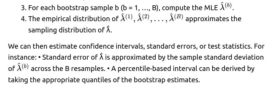
Pitfalls: • The bootstrap can be computationally intensive for very large datasets, though the exponential distribution is fast to sample from. • The method assumes that the parametric form (exponential) is correct. If it is not, bootstrapping around that assumption might be misleading.

Follow-up Question: What if λ itself varies over time, violating the assumption of a constant rate?

In many real-world applications (e.g., customer churn over a product lifecycle, machine failure rates over aging cycles), the rate parameter may not be constant. The exponential model assumes a constant hazard λ, which might not match time-varying hazard rates.

To handle time-varying rates: • Piecewise Exponential Model: Partition the timeline into segments (e.g., [0, 1), [1, 2), etc.), each with its own rate parameter λᵢ. In each segment, assume an exponential distribution with parameter λᵢ. You then estimate multiple λᵢ values, effectively creating a stepwise hazard function. • Weibull or Cox Proportional Hazards: These are more flexible survival analysis frameworks that allow for time-varying hazard functions or incorporate covariates that can change the effective rate. • Nonparametric Methods: Kaplan-Meier estimates can be used for analyzing the survival function without strictly assuming an exponential form.

Pitfall: • Using a single λ for data that clearly have changing rates over time leads to biased or poor fits. The memoryless property is specifically for constant rate processes. If that property is evidently broken, the exponential assumption is no longer valid.

Follow-up Question: Could we employ robust estimation techniques if the data has outliers?

Although outliers in lifetime data might be less common than in other contexts, occasionally you see extremely long or short lifetimes that do not fit the typical distribution pattern. MLE for exponential distributions can be sensitive to outliers, especially if n is small. If a single or few extremely large lifetimes appear, the sum ∑(tᵢ) becomes much larger, pushing λ̂ downward.

Robust estimation approaches: • Winsorizing or trimming extreme values to reduce their undue influence. • Bayesian approach with a prior that limits how extremely large or small λ can become. • Using a heavier-tailed distribution (like a Gamma distribution) if outliers are genuine and indicate tail behavior not compatible with an exponential form.

Pitfall: • Blindly removing or trimming outliers might remove genuine extreme observations. This might improve the “fit” but degrade real predictive performance if, indeed, true rare but large lifetimes occur in the real process.

Follow-up Question: How do we connect continuous exponential models to their discrete-time analogs?

In discrete time settings, the geometric distribution is the analogue to the continuous exponential distribution in that both exhibit the memoryless property. In continuous time, the exponential distribution is memoryless; in discrete time, the geometric distribution is memoryless.

If you observe data in discrete intervals (e.g., each day or week you check if a customer churned), you might approximate the time-to-event using a geometric distribution with parameter p. The relationship between λ and p can be made by considering: • p ≈ 1 − e^(−λΔt), where Δt is the length of each discrete time step.

When Δt is small, p is small, and the geometric distribution’s parameter p is roughly λ times the time-step length. Estimating p via MLE in a geometric model leads to p̂ = number_of_events / total_trials_in_which_they_could_occur. This parallels λ = n / ∑(tᵢ), though the details differ due to discrete vs. continuous formulations.

Pitfall: • Mixing up discrete and continuous data can produce misleading interpretations. If you treat effectively discrete data as continuous, or vice versa, your estimates might not align with how the process actually operates.

Follow-up Question: How do we reconcile domain expertise with purely data-driven estimation of λ?

Sometimes domain knowledge about the process generating the lifetimes can be a powerful guide. For instance, engineering experts might know that a particular machine part has an expected lifetime around 50 hours, or marketing experts might suspect that most churn happens within the first month of subscription.

Ways to incorporate domain expertise: • Use a Bayesian approach with a prior distribution on λ that reflects expert beliefs. • Impose constraints on λ, e.g., you might rule out extremely large or small values based on physical or business constraints. • Check the fit visually (e.g., using survival plots) and see if it aligns with known domain patterns (like an initial “burn-in” or “honeymoon” period).

Pitfall: • Overly strong prior beliefs can drown out the data, leading to a mismatch if the real process differs from expectations. On the other hand, ignoring well-established domain insights can also produce suboptimal or nonsensical models, particularly with small sample sizes.

Follow-up Question: How might we implement a mini-batch or streaming approach to estimating λ for large-scale data?

In massive or streaming data scenarios, storing all lifetimes and computing ∑(tᵢ) directly might be impractical. A mini-batch or streaming approach processes data in chunks. The running formula for λ in a streaming sense can be updated with each new batch of lifetimes:

1. Keep track of a running sum of all observed lifetimes, S, and a running count of the total number of observations, N.

2. Each time a new batch arrives with lifetimes tᵢ^(batch): • Update S ← S + ∑(tᵢ^(batch)). • Update N ← N + (batch size). • Recompute λ̂ ← N / S.

Because the exponential distribution MLE only depends on the sum of all tᵢ and the total count, this approach is straightforward. You do not need to store individual data points—just aggregated statistics.

Pitfall: • Ensure data integrity if partial lifetimes or out-of-order data appear in the stream. Also, if the data are not stationary (i.e., λ changes over time), simply aggregating all data might “average out” different underlying regimes. A sliding window or time-weighted approach might be more appropriate in nonstationary scenarios.

Follow-up Question: How do we implement or fine-tune the exponential MLE in modern deep learning frameworks like PyTorch or TensorFlow?

While we typically do not train just a single exponential distribution in deep learning frameworks, there are scenarios in which one might do so—for instance, to parameterize certain components of a probabilistic model or a survival model.

Implementation details: • Represent λ as a learnable parameter (often the network outputs log(λ) to ensure positivity). • Define the negative log-likelihood for the observed data tᵢ as:

which is simply −ln(L(λ)). • Use automatic differentiation to optimize this negative log-likelihood w.r.t. the parameter λ (or log(λ)). • Because λ must remain positive, applying a softplus or exponential activation can ensure positivity. A common choice is:

λ = exp(θ),

where θ is an unconstrained real parameter learned by gradient-based methods.

Pitfall: • Convergence might be trivial in this case if it’s purely for a single parameter. For more complex architectures involving an exponential distribution as part of a bigger network, you might see gradient issues if the times tᵢ have large ranges. Proper scaling or normalization of tᵢ can help maintain stable gradients. • If partial or censored data is included in the training procedure, you must incorporate the survival term in the loss function (i.e., the negative log survival for censored observations), which complicates the code but is still feasible in frameworks like PyTorch or TensorFlow.

Follow-up Question: Can the exponential MLE approach be used if we aggregate events at the group level rather than the individual level?

Sometimes, the data is not at the granularity of individual lifetimes. Instead, you might have group-level counts of how many customers died (churned) in each time interval but not the exact individual times. In such aggregated data: • You lose the exact Tᵢ. You only know how many events occurred in each bin. • The standard formula λ̂ = n / ∑(tᵢ) no longer directly applies, because we do not have the sum of individual lifetimes.

One approach is to write down the likelihood (or log-likelihood) for grouped or binned data using the fact that the number of events in a time interval is Poisson(λ × length_of_interval) if you assume a Poisson process perspective. Then, you can sum the log probabilities for each bin. The resulting MLE might not have a closed form and would need to be solved numerically.

Pitfall: • If the time intervals are wide, you lose a lot of resolution about exactly when events occurred. The fit might be coarse, or the exponential assumption might fail within each interval. In extreme cases, you may need a piecewise constant approach or a more detailed modeling approach (e.g., maximum likelihood estimation for a Poisson process with intervals).

Follow-up Question: Are there any concerns regarding identifiability when using only a few data points?

Identifiability means the parameter λ can be uniquely determined given the likelihood and the data. Technically, for the exponential distribution with complete, nonzero data, λ is identifiable even from a small sample. However, a very small n (e.g., n=1 or n=2) can lead to: • High variance in the MLE, since ∑(tᵢ) might be driven by very few observations. • Sensitivity to outliers or unusual observations; for instance, with a single data point t₁, the MLE is λ̂ = 1 / t₁, which could be quite large or small if t₁ is short or long.

Pitfall: • Overconfidence in a single or handful of data points leads to naive extrapolation. In real practice, if n is very small, you should incorporate prior beliefs or consider a more robust or Bayesian approach for additional stability. • If any data point is zero or extremely close to zero, the sum might be tiny, pushing λ̂ to an implausibly large value, which might not reflect underlying reality.

Follow-up Question: Is there a connection between MLE for λ in an exponential distribution and partial likelihoods in proportional hazards models?

In survival analysis, especially with the Cox proportional hazards model, we do not assume a particular baseline hazard function’s parametric form; we only assume that covariates multiply the hazard. However, if we specifically assume the baseline hazard is constant, that is effectively an exponential model.

With no covariates, the partial likelihood in a Cox model collapses to the standard likelihood for the exponential distribution. So the MLE for λ in that simplified scenario is the same as what we derive using the standard exponential approach. When covariates are present, the partial likelihood estimates the coefficient vector β for covariates, while the baseline hazard (in a purely exponential baseline scenario) is also estimated.

Pitfall: • When covariates are included, the hazard might no longer be constant across all individuals, even if the baseline hazard is constant. Failing to consider relevant covariates might produce a biased or incomplete view of λ if subgroups have systematically different hazard rates. • The partial likelihood does not always yield a closed-form solution once we incorporate covariates, requiring numerical maximization. But for the simple exponential case, you still have the closed-form expression for λ.

Follow-up Question: Do we need to worry about boundary solutions for λ, such as λ → 0?

In principle, λ > 0. The exponential distribution is undefined at λ = 0. However, in practice, if the data show extremely long lifetimes or possibly no observed events in a time window, you might see the likelihood function push λ to a very small value.

• With standard i.i.d. data and all tᵢ being finite, the MLE formula λ̂ = n / ∑(tᵢ) will never be exactly zero. • If you had some data that implied extremely long lifetimes (or if the total sum is very large), λ̂ can become very small but still positive. • In incomplete data scenarios (e.g., no events observed at all over a certain timescale), it might appear that λ = 0 is the best “fit.” In a strict parametric sense, though, λ = 0 is invalid for an exponential distribution. You would either gather more data or incorporate prior knowledge that real events eventually occur.

Pitfall: • Misinterpretation of a near-zero rate can occur if you are analyzing a partial timeframe in which no events happened. This might lead to incorrectly concluding that λ is effectively 0, while in a longer timeframe events might happen. Always check whether the observation period is sufficient to capture the phenomenon.

Follow-up Question: How does the MLE generalize if we have a shifted exponential distribution?

A shifted exponential distribution introduces a shift parameter δ ≥ 0, meaning the distribution is:

f(t; λ, δ) = λ e^(−λ(t − δ)) for t ≥ δ,

and 0 for t < δ. This might model scenarios where no event is possible before time δ. In that case, we have two unknown parameters: λ and δ.

The MLE derivation for the two-parameter scenario is more involved. Intuitively:

1. δ̂ is often the minimum observed lifetime tₘᵢₙ because shifting any further to the left wouldn’t increase the likelihood, but a shift to the right must not exclude any observed data. This is reminiscent of how location parameters can be handled in certain distributions (like a shifted exponential or Gumbel).

2. Once δ̂ is determined, you effectively fit an exponential distribution with parameter λ to the data tᵢ − δ̂.

Pitfall: • If the data actually does not have a clear lower bound or if some times are genuinely 0, forcing a shift δ > 0 might degrade model accuracy. You need to ensure the concept of a shift parameter aligns with the domain scenario (e.g., a waiting period before a device can fail). • The shift parameter might be confounded with measurement issues or rounding, leading to overfitting if you treat δ as a free parameter for small sample sizes.

Follow-up Question: In practice, could we transform the data to improve numerical stability when computing the MLE?

Sometimes for large or very small tᵢ, summation can be numerically unstable. While the MLE λ̂ = n / ∑(tᵢ) is straightforward, you may: • Work in log-space for partial sums, though that’s less common for a direct ratio. • Use stable summation algorithms (like Kahan summation) to handle large n or wide dynamic ranges of tᵢ. This ensures minimal floating-point rounding errors.

Pitfall: • In typical double-precision arithmetic, you rarely run into catastrophic issues with a single sum, but for extremely large-scale data streams (millions or billions of records with widely varying magnitudes), floating-point accumulation errors can become nonnegligible. • Over-engineering the summation might not be necessary if your data’s range is well within what double precision can handle, but do be mindful if your lifetimes can go from extremely small fractions of a unit to extremely large values.

Follow-up Question: What if the data is heavily skewed, but we still suspect an exponential distribution?

The exponential distribution itself is already right-skewed. If you observe extreme skewness, it might still be consistent with an exponential model, but sometimes the data could be even heavier-tailed than exponential suggests. For instance, you might have a few extremely large values that skew the average significantly.

Tests: • Compare exponential vs. heavier-tailed alternatives (like Pareto or lognormal). • Check Q–Q plots or residual plots to see if the largest lifetimes deviate from the exponential line.

If the tails are significantly heavier than exponential, you may see that a portion of the data is well fit by λ̂, but the largest observations are systematically under-modeled. The MLE formula does not “break,” but the model might be inadequate in describing tail risk or high-lifetime probability.

Pitfall: • Overfitting might occur if you keep trying to adjust λ to capture the tail, but the exponential distribution has only a single parameter. You may systematically underpredict the probability of extremely large observations, leading to misestimation of risk or reliability in practical scenarios.

Follow-up Question: Could the exponential MLE be extended or adapted if you only measure discrete times but treat them as if continuous?

Sometimes data is recorded at discrete intervals (e.g., daily or weekly checks). In principle, this is a discrete-time setting, but you might approximate it as continuous. The question is whether this approximation is valid: • If the sampling frequency is high enough compared to the scale of lifetimes, treating the data as continuous might be a reasonable approximation. • If the data are truly coarse (e.g., only measured once a month, while typical lifetimes are a few days), the approximation might be poor.

You can proceed with λ̂ = n / ∑(tᵢ) if you treat each recorded event time as continuous. This might yield a biased or approximate estimate if the distribution within each discrete bin is not well captured.

Pitfall: • Larger bin sizes can mask the memoryless property if events always appear to occur “just before” the next measurement interval. Ensure your sampling rate is fine-grained enough that continuous-time assumptions are not drastically violated.

Follow-up Question: How do we implement a simple hypothesis test to check if a proposed λ is plausible?

One might want to test a null hypothesis H₀: λ = λ₀ for some known value λ₀:

1. Compute the likelihood of the data under H₀: L(λ₀).

2. Compute the maximum of the likelihood, L(λ̂).

3. Form a likelihood ratio test statistic: −2 ln[L(λ₀) / L(λ̂)].

Under certain conditions (large n, regularity of the exponential family), this statistic approximately follows a chi-square distribution with 1 degree of freedom (because there’s one parameter under test). If the statistic exceeds the critical value for that chi-square distribution (or the p-value is below the chosen threshold), we reject H₀ in favor of λ ≠ λ₀.

Pitfall: • For small sample sizes, the asymptotic chi-square approximation might be inaccurate. In that case, one might prefer exact or simulation-based methods. • If H₀ is on the boundary (e.g., λ₀ → 0), the usual chi-square approximations can fail. You might need specialized boundary-based or exact tests.

Follow-up Question: Do we need to consider spurious local maxima in the likelihood for the exponential distribution?

For the standard exponential distribution with an i.i.d. sample, the likelihood is a concave function in λ (when viewed in the log-likelihood space), so there is a single global maximum at λ = n / ∑(tᵢ). Unlike more complex distributions or mixture models, spurious local maxima do not arise in the single-parameter exponential setting.

However, in more complex expansions (like a mixture of exponentials or a shifted exponential with multiple parameters), local maxima can appear in the parameter space. Then, the simple derivative approach might not yield the unique global maximum, and one typically uses the EM algorithm or advanced optimization methods that can locate multiple local maxima.

Pitfall: • If you incorrectly assume a single global maximum for a mixture of distributions, you might get stuck in a local maximum. Good initialization or multiple random restarts in the EM algorithm helps mitigate that risk for mixture models. For the single-parameter exponential, this concern does not apply in the standard setting.

Follow-up Question: How do we reconcile the interpretation of λ as a rate with actual time units?

If the dataset is in days, then λ has units of “per day.” If it’s in hours, λ is “per hour.” It’s easy to conflate them if you do not keep the units consistent. Always keep track of the time scale.

Example: If we measure the average lifetime of a component in hours, and find λ̂ = 0.02, then the implied mean lifetime is 1 / 0.02 = 50 hours. If we switch to a measurement in days (1 day = 24 hours), the rate in “per day” terms would be λ′ = λ * 24 = 0.48, giving a mean lifetime of about 2.083 days.

Pitfall: • Inconsistent units lead to confusion or incorrectly comparing rates. Domain knowledge might specify lifetimes in months or years for business contexts. Always double-check that you’re applying the correct time scale.

Follow-up Question: Does the exponential distribution’s memoryless property cause any practical paradoxes or misunderstandings?

Yes, a common misunderstanding is the “waiting time paradox” or related illusions where people observe that “since I’ve already waited a while, the chance of waiting much longer should be higher or lower.” For an exponential distribution, the memoryless property states the distribution of the remaining time does not depend on how long you have already waited.

Practical confusion: • In real life, many processes are not strictly memoryless. If you have already waited a long time for a bus, it might indicate that something unusual is happening (breakdown, schedule disruption), so the chance of waiting even longer might be higher than what an exponential assumption would suggest. • In some contexts (like random phone calls in a telecommunication system under stable conditions), the exponential assumption might be a good approximation and the memoryless property holds fairly well in practice.

Pitfall: • Relying on an exponential assumption can lead to underestimation or overestimation of event timing if the real process is not truly memoryless. For instance, mechanical parts might degrade over time, making the hazard rate increase with age—contrary to the exponential distribution’s constant hazard assumption.

Follow-up Question: How to interpret the hazard function and survival function in an exponential distribution context?

For an exponential distribution, the hazard function is constant: h(t) = λ. This means the instantaneous risk of the event happening at time t is the same, regardless of whether you are at t = 0 or t = 10 hours.

The survival function is S(t) = P(T > t) = e^(−λt). So the fraction of items still “alive” (or customers still active) decays exponentially with rate λ.

In business terms, if you are modeling churn with an exponential distribution, the hazard rate λ is the constant per-unit-time chance of a customer leaving. If λ = 0.1 per week, it means any given week, there is a 10% chance the customer churns in that week, independent of how many weeks they have already stayed.

Pitfall: • Real churn processes might exhibit a decreasing hazard (customers that survive the initial onboarding phase are less likely to churn) or an increasing hazard (customers lose interest over time). Thus, a constant hazard might be too simplistic in many real business applications, even though it is a good baseline or starting assumption.