
ML Interview Q Series: Minimum Die Roll Analysis: Calculating Expected Value and Standard Deviation.
Browse all the Probability Interview Questions here.
A fair die is rolled six times. What are the expected value and the standard deviation of the smallest number rolled?
Short Compact solution
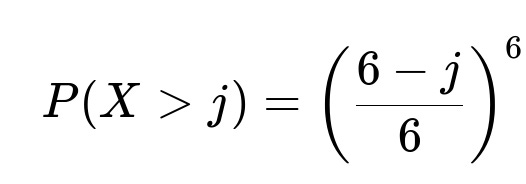
Let X be the smallest number rolled among six independent rolls of a fair die. We note that for each integer j from 0 to 5:
Comprehensive Explanation
Define X as the minimum (smallest) outcome observed when rolling a fair six-sided die six independent times. Each outcome can be any integer from 1 to 6 with equal probability 1/6.
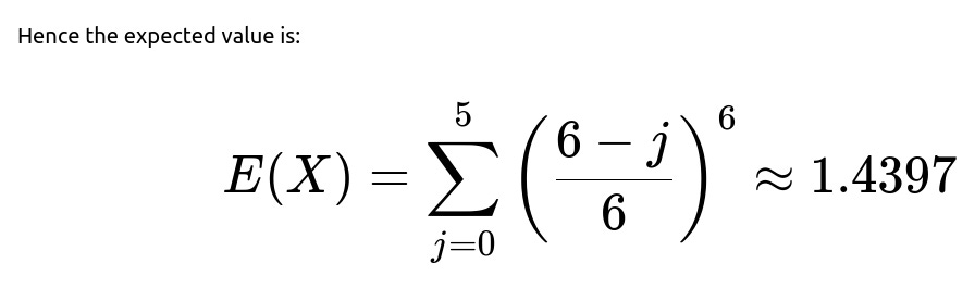
Understanding how to compute E(X): We observe that for a particular j (where j = 0, 1, 2, 3, 4, 5), the event X > j means “the smallest number rolled is strictly greater than j.” Because each die roll is 1 through 6 with probability 1/6 each, the probability that a single roll is greater than j is (6 - j)/6. For all six rolls to be greater than j simultaneously, the probability is ((6 - j)/6)^6. Summing this probability over j = 0 to 5 gives E(X), because:
E(X) can be written as sum_{j=0..5} P(X > j).
This is a useful identity: E(X) = sum_{m=1..∞} P(X >= m). But here, since X cannot exceed 6, we adjust the summation to a finite range of j.
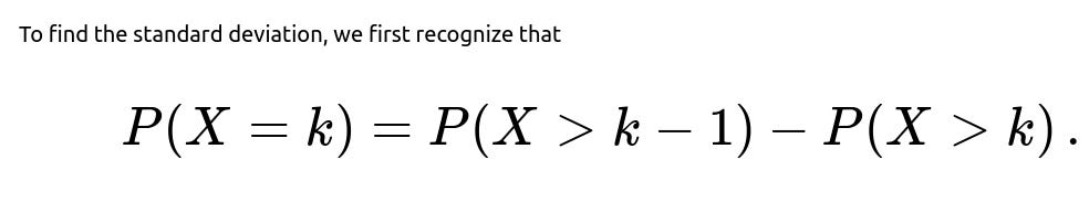
Deriving the distribution P(X = k): We note that P(X = k) is the probability that the smallest number is k. This can be expressed as:
The smallest number is strictly greater than k-1, minus the probability the smallest number is strictly greater than k.
In other words, P(X = k) = P(X > k - 1) - P(X > k).
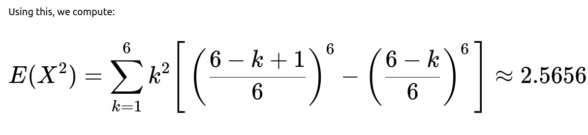
Once we have P(X = k), it is straightforward to compute E(X^2) = sum_{k=1..6} k^2 * P(X = k). The result from the snippet’s calculation is approximately 2.5656.
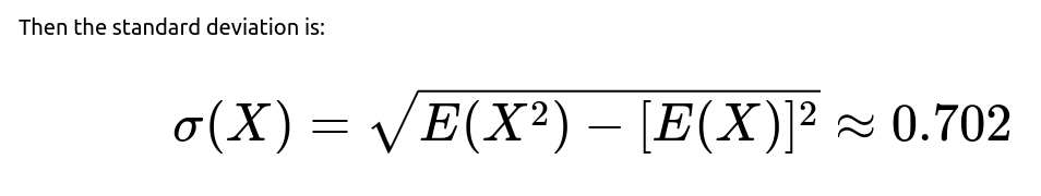
Finally, we use the standard formula for variance Var(X) = E(X^2) - [E(X)]^2. Taking the square root yields the standard deviation sigma(X) = sqrt(Var(X)) ≈ 0.702.
In summary, the smallest number rolled is quite likely to be on the lower side of the 1 through 6 range, which is reflected in the expectation being about 1.44. The spread of this distribution (standard deviation ~ 0.70) is relatively small.
Potential Follow-Up Questions
Could we approach this using a direct counting method?
Yes. Instead of using the “greater than j” approach, we could directly count the number of outcomes (in the sample space of 6^6 total outcomes) for which the minimum is exactly k. Specifically:
To have the minimum be exactly k, all six rolls must be >= k, and at least one roll must be equal to k.
We can count the number of ways all six rolls are in the set {k, k+1, …, 6}, then subtract the ways all six rolls are in {k+1, k+2, …, 6}.
This direct counting approach leads to the same probability distribution P(X = k). It is a more combinatorial viewpoint but ends up with the same final formula.
What is the distribution of X in a more general sense?
X has a discrete distribution supported on {1, 2, 3, 4, 5, 6}. For a general n-sided die rolled m times, we can generalize:
The probability that the minimum is greater than j is ((n - j)/n)^m.
Hence E(X) = sum_{j=0}^{n-1} ((n - j)/n)^m.
You can similarly compute P(X = k) for k = 1..n and then derive higher moments, such as E(X^2), from these probabilities.
How can we verify the solution numerically?
A simple Python script can empirically estimate E(X) and sigma(X) via simulation:
import random
import statistics

def simulate_smallest_roll(num_experiments=10_000_00):
    results = []
    for _ in range(num_experiments):
        rolls = [random.randint(1, 6) for _ in range(6)]
        results.append(min(rolls))
    return statistics.mean(results), statistics.pstdev(results)

mean_est, std_est = simulate_smallest_roll()
print("Estimated E(X):", mean_est)
print("Estimated σ(X):", std_est)
Running this simulation with a sufficiently large number of trials should give an estimated mean near 1.44 and standard deviation near 0.70.
How does the smallest roll scale if we roll the die more or fewer times?
If you roll the same fair six-sided die more than six times, the minimum tends to be smaller on average. For instance, if you roll it 10 times, it becomes more likely that at least one roll is a 1. Conversely, if you roll only three times, the smallest number is not as likely to be as low as when rolling six times, so you would get a larger expected minimum. Formally, if you roll n times, the probability that the minimum exceeds j is ((6-j)/6)^n, which decreases as n grows, pushing the expected minimum downward.
Could we directly extend this idea to the largest number rolled?
Yes. By symmetry, the largest number Y among six rolls has distribution:
P(Y < j) = (j/6)^6 for j in {1, 2, 3, 4, 5, 6}.
E(Y) = sum_{j=0..5} P(Y > j).
However, this largest-value scenario is often simpler if you note that Y = 6 - W, where W is the minimum of six independent “inverted” dice rolls. There are neat parallels, but the computations mirror the same logic used for the minimum.
All these points show how understanding the distribution of extrema (minimum/maximum) in a finite discrete setting is straightforward once you employ complementary probability and summation techniques to derive either an explicit formula or a direct counting approach.
Below are additional follow-up questions
If the dice were not fair, how would that affect the distribution and calculation of the smallest number?
In many real-world scenarios, dice might be biased so that certain faces appear more or less frequently than others. When the die is not fair, each face i in {1, 2, 3, 4, 5, 6} might have a different probability p(i), such that p(1) + p(2) + … + p(6) = 1. The previous derivations for X, the smallest roll, assume a uniform probability of 1/6 for each face, so we would need to adjust all computations to account for the new probabilities.
Detailed reasoning
Let p(i) be the probability that a single roll shows face i.
The probability that a single roll is strictly greater than j (for j in {0, 1, …, 5}) is sum of p(k) for all k > j.
Hence P(X > j) = [sum of p(k) for k > j]^6 because we need all 6 rolls to be greater than j.
From there, we can compute E(X) = sum_{j=0..5} P(X > j), or we can explicitly compute P(X = k) by noting:
P(X = k) = P(all rolls >= k) – P(all rolls >= k+1).
But here, “all rolls >= k” must be carefully computed as [sum_{m = k..6} p(m)]^6.
Subtle pitfalls
If one or more faces have zero probability (for instance, the die never lands on face 3), then we have to account for the fact that X cannot possibly be 3.
Numerical stability might be a concern if p(i) is extremely small or extremely large, especially when raised to the 6th power, as floating-point underflow or overflow might occur in actual code implementations.
Verification with real-world data can be less intuitive if the bias is not known precisely, so we might rely on partial knowledge or an estimate of each p(i).
How do we handle the continuous analog of this problem?
Instead of rolling a discrete die, consider sampling from a continuous distribution X on an interval, for instance from a Uniform(0, 1) distribution, repeated 6 times. Then the “smallest value” among these 6 samples, call it Y, can be approached with continuous probabilities.
Detailed reasoning
For a Uniform(0, 1) random variable U, P(U > x) = 1 – x for x in [0, 1].
With 6 i.i.d. samples, P(all 6 samples > x) = (1 – x)^6 for x in [0, 1].
Thus P(Y > x) = (1 – x)^6, so P(Y <= x) = 1 – (1 – x)^6, which is the CDF of Y.
We can find the PDF by taking the derivative: f_Y(x) = 6(1 – x)^5 for x in [0, 1].
From there, E(Y) = integral_{0..1} x * 6(1 – x)^5 dx. This integral can be solved by standard calculus techniques (it yields 1/7).
The standard deviation can also be computed by integrating x^2 * 6(1 – x)^5 dx and then subtracting [E(Y)]^2.
Subtle issues
Unlike the discrete case, there is no finite set {1, 2, 3, 4, 5, 6}. Instead, the domain is continuous.
In many practical cases (e.g., measuring times, distances, etc.), the distribution might not be exactly uniform, so the exact form of the PDF or CDF must be used for the general approach.
Could we derive closed-form expressions for E(X^n) in general?
This question targets the computation of higher moments (for instance, E(X^3), E(X^4)) or arbitrary powers. Such expressions are indeed possible to derive, though the sums become more involved.
Detailed reasoning
We know E(X^n) = sum_{k=1..6} k^n * P(X = k) for the discrete 6-sided die case.
P(X = k) can be expressed in terms of (6 – k + 1)/6 and (6 – k)/6 raised to the 6th power.
In principle, we can keep summing k^n times the difference of those terms. As n gets larger, it can become more computationally intensive, but still feasible for a finite range of k from 1 to 6.
For continuous distributions, we rely on integrals of the form E(X^n) = ∫ x^n f_X(x) dx. For the minimum, we can use the PDF derived from F_X(x) = P(X <= x).
Potential pitfalls
Summation mistakes and boundary conditions are common errors when implementing code for E(X^n).
For large n, numerical precision can be an issue if certain terms are subtracted from each other in ways that cause floating-point round-off.
What if we are interested in the number of times the minimum value appears?
Another nuanced question is: if we know X is the minimum, how many of the six rolls equal X? This leads to a secondary random variable—let’s call it Y, the multiplicity of the smallest face.
Detailed reasoning
Once X = k is known, we want to know how many times the result k occurs among the 6 rolls.
P(X = k) is the probability that the minimum is k. Conditional on that event, the distribution of exactly how many rolls are equal to k can be approached via combinatorial arguments:
We know no roll can be less than k.
At least one roll must be k.
The remaining 5 rolls can be either k or above k, subject to the condition that at least one roll is exactly k.
Alternatively, we can compute unconditionally by enumerating: how many ways to place r occurrences of k, and each of the other 6 – r outcomes is in {k+1..6}, ensuring that at least 1 occurrence of k is present. Then we sum over possible values of r.
Subtlety
This is relevant in some gaming situations where you might not only want to know the smallest roll but also how many times that smallest face appeared (e.g., to break ties or to decide certain rules).
The calculations can be error-prone if we forget to exclude the scenario that might inadvertently allow values below k or if we incorrectly include the scenario with zero rolls = k.
How do we handle large numbers of dice rolls in a practical simulation?
Rolling 6 dice is straightforward, but in certain applications—like Monte Carlo or large-scale probability studies—we might roll 10,000 dice and ask for the smallest outcome.
Detailed reasoning
For a large number n of dice, the exact formula for P(X > j) = ((6 – j)/6)^n can become extremely small for j > 1. In fact, the probability that the minimum is bigger than 1 can vanish quickly for large n.
In practical terms, for large n, X is almost surely 1. This means the expected value E(X) will be very close to 1, and the standard deviation will be correspondingly small.
Potential pitfalls
Floating-point underflow can happen if we do direct calculations with ((6 – j)/6)^n for large n. Instead, it might be better to use a log-based approach to avoid numerical underflow.
In a real programming scenario, it is easy to get 0.0 due to floating-point limitations, thus losing all resolution in the probabilities.
What if the dice outcomes are dependent in some manner?
The original derivation hinges on the independence of the six dice rolls. If the dice were somehow correlated—e.g., we always force at least two rolls to match or we have a device that couples dice physically so that if one is high the other tends to be low—the distribution of the minimum changes.
Detailed reasoning
P(X = k) for a correlated scenario cannot be factorized simply into products of single-roll probabilities.
We would need the joint probability distribution of all six outcomes. Then we could find the probability that min = k by summing over all 6-tuples (x1, x2, x3, x4, x5, x6) such that each xi >= k and at least one xi = k.
This is much more complex and typically no closed-form solution for general correlations. In certain specialized correlation structures, partial solutions may be possible.
Subtlety
In real-world games, dice are usually designed to be as independent as possible, but mechanical or production flaws can introduce minor correlation. This is often negligible, but in a highly sensitive scenario, ignoring minor correlation can skew the results.
Could the concept of the smallest number generalize to other order statistics like the second smallest or the median?
Yes, we can generalize. The k-th order statistic among 6 i.i.d. discrete random variables is the k-th smallest value. This problem specifically addresses the 1st order statistic (the minimum). Similar logic can find the 2nd smallest, 3rd smallest, etc.
Detailed reasoning
For the k-th smallest, we typically use the formula from order statistics: P(X_(k) = m) = sum_{all combinations} [the probability that exactly k–1 of the rolls are < m, exactly 1 roll equals m, and the rest are >= m].
In the discrete case with 6 dice, it often boils down to combinatorial sums or differences of terms involving binomial coefficients.
For the continuous case, well-known Beta-distribution relationships arise from the classical order statistics formula for i.i.d. Uniform(0, 1).
Potential pitfalls
Many interviewees mix up the difference between “the k-th smallest” and “the number of times the smallest face appears.” They are conceptually distinct.
The counting can grow more complicated for the middle order statistics, though the approach remains systematic.
In practice, how might these results be useful beyond simple dice games?
Though it is a seemingly trivial dice question, the idea of the minimum of multiple “samples” arises in many applied fields.
Detailed reasoning
In industrial quality control, if you take multiple measurements, the smallest reading might indicate a possible shortfall or defect threshold.
In reliability engineering, if you test 6 components in parallel, the system fails when the first component fails (the “minimum time to failure” concept). The same formulas for the distribution of the minimum apply, though the “die faces” become continuous time-to-failure distributions.
In finance, if you consider 6 different instruments’ returns in a single period, the smallest return might be relevant for a worst-case scenario or risk measure.
Edge cases
If the domain of each measurement is finite or infinite, we have to adapt the formulas from the discrete to the continuous domain.
If the measures are not identically distributed, even though we might still treat them as independent, each sample might have a distinct distribution, complicating the minimum’s distribution (since not all draws come from the same probability law).