ML Interview Q Series: Mitigating Vanishing & Exploding Gradients: ReLU, Initialization, Batch Norm, Residual Connections.

📚 Browse the full ML Interview series here.

1. Vanishing/Exploding Gradients: Deep neural networks can suffer from the vanishing gradient problem. What causes vanishing (or exploding) gradients when training very deep networks, and what techniques can help mitigate this issue? Discuss factors like certain activation functions (sigmoid/tanh) and initialization, and methods such as ReLU activations, careful weight initialization (Xavier/He), batch normalization, or residual connections.

Vanishing and exploding gradients are a common challenge in deep neural networks. These phenomena are intimately related to how gradients backpropagate through many layers. In very deep architectures, small deviations in factors such as activation functions, weight initialization scales, or network depth can lead to gradients either becoming very small (vanishing) or very large (exploding) as they flow back through all the layers.

Causes of Vanishing/Exploding Gradients

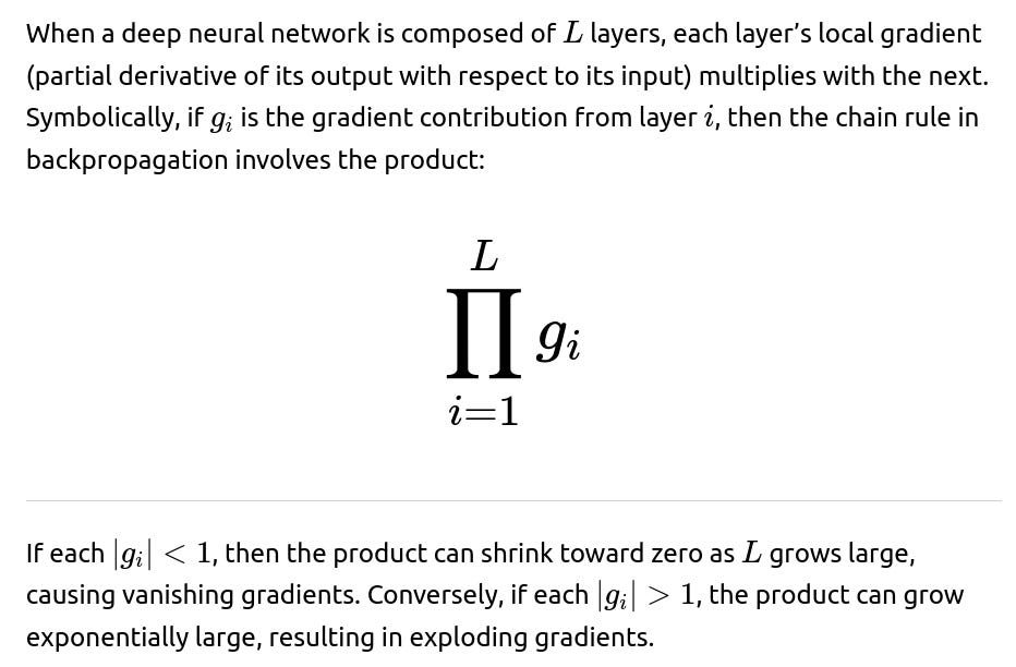
One core cause is the repeated multiplication of gradients through each layer when backpropagating. If these multipliers are less than 1 in absolute value, the gradient diminishes exponentially with depth. If they are greater than 1, the gradient magnifies and may explode.

Sigmoid or tanh activation functions can exacerbate this. In these functions, a large portion of the input domain saturates to near-constant outputs, which correspond to near-zero slope in those regions. When the slope is near zero, backpropagated gradients become extremely small and vanish. If weights are poorly scaled, the gradient can also explode.

Improper weight initialization can create large or very small output magnitudes at each layer. If the weights are too large, outputs and gradients explode; if they are too small, they vanish. Early training steps in such a network often fail or become unstable.

Techniques to Mitigate Vanishing/Exploding Gradients

Activations such as ReLU (Rectified Linear Unit) help address vanishing gradients by providing a constant slope of 1 in the positive domain. Modern variants like Leaky ReLU or ELU also avoid saturating to zero in the negative domain, offering a steadier gradient flow.

Careful weight initialization, such as Xavier (Glorot) or He initialization, sets the variance of the weights in a way that better preserves the scale of signals across layers. The objective is to maintain stable activations and gradients throughout the network depth.

Batch normalization normalizes the distribution of activations at each mini-batch, reducing internal covariate shift. This tends to keep the gradients at manageable scales.

Residual connections (or skip connections) in architectures such as ResNet allow gradients to flow directly from deeper layers to shallower layers. This bypasses some of the repeated multiplications and alleviates vanishing gradients.

Hyperparameter selection (learning rate, weight decay, etc.) can also help. A well-chosen learning rate avoids extremes of exploding gradients or extremely slow convergence.

Connections to Mathematical Expressions

Balancing the magnitude of these gradients via improved activation functions, weight initialization, and other architectural designs is critical.

Subtle Real-World Considerations

Even with modern techniques, deep networks can still experience some form of gradient instability if hyperparameters are suboptimal. For example, if a ReLU network is initialized with an overly large variance, the outputs might blow up in early layers. If the learning rate is too high, weights can also diverge quickly. Furthermore, batch normalization can interact with certain dropout rates to produce unexpected behaviors, especially if the batch size is small, complicating the gradient flow. Residual connections also introduce interplay between the skip path and the main path, so the network might rely heavily on skips if the main path is not carefully managed, potentially underutilizing the representational capacity of deeper layers.

How might switching from sigmoid to ReLU activations address vanishing gradients?

Sigmoid functions saturate for large positive or negative inputs, yielding near-zero derivatives in those regions. This means the gradient is nearly zero for many input values, causing vanishing gradients. ReLU addresses that because in the positive domain, it has a constant derivative of 1, maintaining gradient flow. Although ReLU sets negative inputs to zero, it at least has a non-zero gradient for all positive inputs. This difference often substantially reduces vanishing gradients in practice. A negative input passing through ReLU becomes zero, which can theoretically lead to “dying ReLUs,” but the percentage of completely “dead” neurons is often lower in well-initialized networks compared to the large-scale saturation often observed with sigmoid or tanh.

Potential pitfalls include the possibility of having too many negative inputs so that a portion of ReLU neurons do not update. Techniques like leaky ReLU, ELU, or parametric ReLU can help alleviate that.

Why is careful weight initialization important to mitigate these problems?

Improper initialization can place the activations of many neurons in regions where the gradient is extremely small or extremely large. With sigmoid or tanh, if weights are large, the input to the activation saturates and the gradient can vanish. If weights are very small, the output is near zero, so the network might fail to learn useful representations. Furthermore, large or unbalanced initial weights can cause an explosion of forward or backward signals.

Xavier (Glorot) initialization tries to maintain a consistent signal variance as it passes forward and backward by setting the initial variance of weights in a layer as a function of both the incoming and outgoing layer sizes. He initialization modifies this idea for ReLU-based networks, taking into account that half the outputs will be zero. These initializations reduce the likelihood that gradients vanish or explode in early training.

What is the role of batch normalization?

Batch normalization normalizes intermediate activations in each mini-batch to have zero mean and unit variance (then learns scale and shift parameters). This keeps the magnitude of the inputs to subsequent layers more consistent. By normalizing hidden activations, large or small fluctuations that cause gradient instability are reduced.

It also mitigates the internal covariate shift: as network parameters update, the distribution of layer inputs changes, making it harder to train. Batch normalization counters this by ensuring the inputs to each layer are relatively stable in their mean and variance across training iterations.

One subtlety is that batch normalization introduces additional complexity if your batch size is small, since the statistics used to normalize might not be reliable estimates of the true distribution. There are alternative normalization methods such as Layer Normalization or Group Normalization that do not rely on batch statistics in the same way.

How do residual connections help with vanishing gradients?

Residual connections, introduced in ResNets, enable the gradient from deeper layers to bypass intermediate transformations by “skipping” certain layers. This helps preserve gradient magnitude during backpropagation. Even if certain layers have near-zero local gradients, the skip connection can carry the gradient from deeper layers directly to the shallower ones.

When the residual block is formulated as

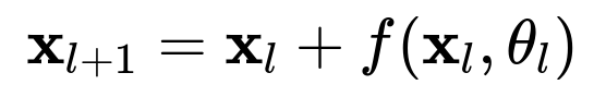
then backpropagating the gradient involves both the derivative of f and a pass-through path of derivative 1 for the identity connection. This reduces the risk that the overall gradient product is too small, thus alleviating vanishing gradients and enabling significantly deeper networks.

How might the choice of optimizer or hyperparameters influence vanishing/exploding gradients?

Very high learning rates can cause updates that overshoot minima, leading to runaway gradients. Momentum-based methods can compound the issue if the gradient direction changes abruptly. In an extreme case, weights can explode in magnitude from one iteration to the next. Conversely, a learning rate that is too low risks very slow training, potentially exacerbating mild vanishing gradient problems, as each update might be far too small.

Optimizers like Adam dynamically adjust the effective learning rate for each parameter, reducing the risk of exploding gradients. Gradient clipping is another strategy that prevents any given gradient vector from exceeding a specified threshold, effectively capping the maximum norm. This protects the network from extremely large steps.

Could skipping normalization or skipping residual connections still train a deep network successfully?

In principle, yes, but it’s difficult in practice. Very deep networks without any forms of normalization, skip connections, or advanced initialization might still learn if well-tuned or if the architecture is not excessively deep. However, the training process would be more delicate and prone to these gradient instabilities. In real-world scenarios, scaling beyond moderate depths typically demands some combination of advanced initialization, normalization, or skip connections.

What might happen if a network with ReLU activations is initialized incorrectly?

If the initial distribution of weights is too large, many neurons might receive large positive or negative inputs. Some of them might saturate on the positive side, leading to quickly exploding activations in forward pass. Others might produce large negative outputs that are clamped to zero by ReLU, effectively leading to no gradient updates for those neurons. Over multiple layers, such an imbalance can cause either vanishing or exploding patterns and hamper training altogether.

Setting a smaller variance could lead to an extremely large percentage of ReLU neurons immediately producing zero. If many neurons are “dead” from the start, training might never escape a suboptimal region. That’s why He initialization (or a variant) is typically favored for ReLU-based networks, as it specifically accounts for the proportion of “active” ReLU outputs.

How does gradient clipping help in practice?

Gradient clipping is a practical technique, often used in RNNs and LSTM networks, where exploding gradients are especially common. After computing the gradients for all parameters, one checks the norm of the entire gradient vector. If it exceeds a threshold, it is scaled down to match that threshold. This prevents any one update from being too large.

An example in code:

import torch

# Suppose loss has been computed
loss.backward()

# Gradient clipping
max_norm = 1.0
torch.nn.utils.clip_grad_norm_(model.parameters(), max_norm)

# Proceed with optimizer step
optimizer.step()

This approach does not directly address the root cause of exploding gradients, but it prevents them from causing catastrophic weight updates.

How does the vanishing gradient phenomenon relate to RNNs specifically?

Recurrent Neural Networks repeatedly multiply gradients through time steps, so they can be thought of as having very deep structures unrolled over time. If the recurrent weight matrix leads to eigenvalues less than 1 in magnitude, repeated multiplication can vanish over many time steps. If eigenvalues are greater than 1, the gradients can explode. LSTM and GRU architectures include gating mechanisms that help control these repeated multiplications. They are designed to mitigate vanishing gradients by allowing better gradient flow over longer sequences, though they can still face exploding gradients, often handled with clipping.

What are realistic best practices for designing very deep networks to avoid vanishing or exploding gradients?

Using ReLU or its variants as the activation function in most layers, combined with He or Xavier initialization, is a standard practice. Batch normalization is commonly inserted between convolutional or fully connected layers. Residual connections are standard in many modern architectures like ResNets, DenseNets, or Transformers (which have skip connections in their attention blocks).

One typically couples these architectural choices with a well-chosen optimizer such as Adam or RMSprop, a suitable learning rate schedule (e.g., warm restarts or cosine decay), and possibly gradient clipping in cases of recurrent architectures or whenever the gradient norm might spike.

Having a well-structured design with skip connections and normalization is almost a default approach for successful training at scale. Regular checks of gradient statistics (e.g., their mean or norm in each layer) can provide insight into whether vanishing or exploding phenomena occur during training.

---

Below are additional follow-up questions

What are some potential pitfalls of using very large batch sizes on gradient stability, and could this contribute to vanishing or exploding gradients in practice?

Large batch sizes can lead to smoother gradient estimates because each mini-batch is a more faithful approximation of the full dataset’s gradient. However, there are subtle pitfalls:

When a batch is very large, the step size (learning rate) might need to be adjusted more carefully. Sometimes people scale the learning rate by the batch size, but this can cause explosive updates if the scaling is too aggressive, especially at the very beginning of training. Even with stable activations, an overly high global learning rate can trigger divergences in the first few epochs.

Large batches reduce the frequency of parameter updates for a given epoch, and if the network’s parameter space is complex, fewer updates can slow down the training dynamics. The network might find a region of parameter space that is flatter but not necessarily better at generalization. If the chosen learning rate is too high, occasionally the combination of a large batch and a large update can push weights into a regime of activation saturation or extremely large outputs, leading to exploding gradients in subsequent steps.

Additionally, if the architecture contains layers with poorly calibrated initialization or extremely sensitive layers (like recurrent layers with gating), the large-batch training might mask early signs of gradient explosion or vanishing until the model reaches a point of irrecoverable instability. Smaller batches, on the other hand, might spot these signs earlier (due to higher variance in gradients) and either adapt or fail quickly.

To mitigate these issues, practitioners often adopt techniques like learning rate warm-up, where the learning rate is slowly increased over the initial iterations when training with large batch sizes. This helps ensure that gradients and weights remain stable during early training stages.

How might dropout impact vanishing or exploding gradients, and are there special considerations when combining dropout with batch normalization?

Dropout randomly zeros out a subset of neuron outputs during training. This can act as a form of regularization, but it also changes the distribution of activations. When dropout is present, each forward pass sees a slightly different network topology.

One potential impact on gradient stability is that dropout can sometimes amplify or mute signals stochastically. If many key neurons in one layer are dropped, the next layer might receive significantly smaller input signals, contributing in a minor way to vanishing gradients in certain timesteps. However, since dropout is random and typically used with a moderate rate, it usually does not systematically cause vanishing gradients. Rather, it can slightly increase gradient variance.

In conjunction with batch normalization, the distribution of activations can be different for training (with dropout enabled) versus inference (when dropout is typically disabled). Because batch normalization relies on the mean and variance of activations, these statistics might become less stable if dropout has a large effect on the distribution. In extreme cases (e.g., high dropout rates or very small batch sizes), the mismatch between training and inference distributions can inadvertently contribute to either exploding or diminishing activations when dropout is turned off at test time. Carefully tuning dropout probability, batch size, and the momentum in batch norm helps avoid these issues. Some architects place dropout after batch normalization instead of before, but the best approach can vary by architecture.

How can layer normalization or group normalization help with vanishing or exploding gradients, especially compared to batch normalization in situations where batch sizes are very small or data is highly non-i.i.d.?

Layer normalization normalizes across the neurons in a single layer for each sample independently, instead of across the samples in a mini-batch. Similarly, group normalization splits channels into groups and normalizes within each group. These methods avoid relying on batch-level statistics, which can be unreliable when the batch size is small or the data in each mini-batch is not i.i.d.

By normalizing per sample (layer norm) or per sample group (group norm), these approaches stabilize the activations and their gradients within each forward and backward pass. This is extremely useful in scenarios such as reinforcement learning or certain NLP tasks where data might be sequentially dependent or batched in small sizes for memory reasons.

Without stable normalization, the repeated multiplications through many layers can accumulate small numeric differences, leading to either vanishing or exploding gradients. Layer or group normalization helps ensure the scale of activations does not drift too far from a stable range during forward propagation, thereby confining gradients to a manageable scale in backpropagation.

Potential pitfalls include computational overhead if implemented naively, and also the risk that normalizing each sample’s features too aggressively could remove meaningful scale differences. In practice, however, these normalization techniques often improve training stability significantly for deep models when batch normalization is less effective.

Could certain regularization methods like or weight penalties exacerbate vanishing gradients in deeper networks?

regularization (weight decay) shrinks weights continuously, while regularization encourages sparser weights by pushing small weights toward zero more aggressively. In principle, moderate regularization helps keep the parameter magnitudes under control, reducing the likelihood of exploding gradients.

However, in a very deep network on the brink of vanishing gradients, excessive weight decay might push the weights even smaller in magnitude, contributing to smaller intermediate signals. Since backpropagation depends on these signals, a heavy penalty could further reduce gradient magnitudes and slow learning, effectively reinforcing vanishing gradients. regularization, while forcing sparsity, could zero out many connections if the gradient flow is already weak.

A balanced approach is often best: mixing suitable normalizing activation functions, proper initialization, and moderate weight regularization. A too-aggressive regularization regime can undermine training signals in a deep architecture, particularly if the baseline gradients are already small.

How do advanced architectures like DenseNets manage gradient flow differently from ResNets, and could they handle vanishing gradients even better?

DenseNets create direct connections from each layer to every subsequent layer within a block. This means the feature maps of preceding layers are concatenated and passed into deeper layers. Consequently, each layer receives a consolidated set of features, including those from the very early layers. By design, this architecture helps gradient flow because the chain of transformations from early layers to deeper layers is shortened.

Where a ResNet provides an additive skip connection from layer l to layer l+2, a DenseNet effectively provides multiple “skip lines,” one from layer l to l+1, l+2, ..., up to the final layer in the block. This direct connectivity pattern can reduce the risk that gradients vanish by allowing them to flow back directly to earlier layers.

A potential drawback is the significant memory overhead, since the number of feature maps grows with each layer. Also, the risk of exploding gradients could theoretically increase if the concatenated features cause an outsized scale of activations, but in practice, careful design with smaller growth rates (number of new feature maps per layer) keeps the network stable. Moreover, batch normalization is almost always used in DenseNets, further controlling activation scales.

Are there any scenarios where using sigmoid or tanh might still be favorable despite their risk of causing vanishing gradients?

While ReLU (and variants) have become standard, sigmoid and tanh functions can still be useful in certain networks, especially in output layers for tasks like binary classification (sigmoid) or zero-centered tasks (tanh). Also, gated recurrent units like LSTMs rely on sigmoid or tanh inside their gating mechanisms, though these architectures are specifically designed to mitigate the vanishing gradient problem through additional internal gating and memory cells.

In some specialized contexts (e.g., probabilistic modeling or certain energy-based models), sigmoid or tanh might be mathematically more natural. Proper initialization, careful architecture choices, and gating (in recurrent networks) can help counteract the typical saturation issues. The key is that if a design requires sigmoid or tanh for theoretical or functional reasons, other protective measures such as gating, residual connections, gradient clipping, or advanced initialization help maintain stable training.

Could activation quantization or reduced precision arithmetic (like FP16) exacerbate vanishing or exploding gradients?

When using mixed-precision or reduced-precision arithmetic (e.g., FP16), numerical ranges become narrower. If gradients become very small (close to the minimum representable number in FP16), they may underflow to zero, accelerating vanishing gradients. Conversely, if a gradient is too large, it might overflow, “nan” out, or saturate at the maximum representable magnitude in FP16, contributing to exploding gradients.

Frameworks like PyTorch or TensorFlow often employ loss scaling when training in FP16. This multiplies the loss by a scale factor to keep gradients in a representable range. If an overflow is detected, the scale factor is reduced. This dynamic scaling helps mitigate many precision-induced gradient issues. Nonetheless, improper or inconsistent scaling can still cause silent gradient vanishings or explode the updates.

In practice, if the network is carefully designed (with skip connections, normalization, etc.) and the training code uses well-tested mixed-precision routines, these problems are usually minimal. However, in corner cases (like extremely deep RNNs or unbounded activation growth), half-precision can amplify gradient instability, and some engineers prefer to revert to full precision training for particularly difficult models.

In the context of graph neural networks (GNNs), how can vanishing or exploding gradients manifest differently, and what architectural methods mitigate them?

Graph neural networks have layers that aggregate features from neighbors in a graph. Each layer typically involves some combination of message passing, summing or averaging neighbor embeddings, and applying a learnable transformation (e.g., a linear layer or MLP). Over many layers, signals can diffuse across the graph. If the graph is large or has nodes with high degree, repeated aggregations could cause either very large or very small signals.

Exploding gradients could arise if neighbor embeddings become repeatedly amplified through aggregation and non-linear transformations, especially in graphs with hubs having extremely high connectivity. Meanwhile, vanishing gradients might happen if repeated averaging over large neighborhoods dilutes signals or if activation functions saturate.

Common mitigations include skip connections across GNN layers (similar to ResNets, often called Jumping Knowledge networks), normalization layers such as GraphNorm or LayerNorm adapted for GNNs, and careful initialization of graph convolution parameters. Some GNN variants also incorporate gating (like GRU gating) within message-passing steps, helping maintain gradient flow.

Could multi-task learning, where multiple losses are backpropagated through a shared backbone, lead to gradient explosion or vanishing issues if not carefully balanced?

Multi-task learning shares a backbone of layers among different tasks, each with its own loss component. The total loss might be a weighted sum of individual task losses. If one task’s loss is significantly larger or has much larger gradient magnitudes, it can dominate the training signal. This can trigger explosion of weights relevant to that task, while other tasks receive comparatively tiny updates and effectively vanish in the competition for gradient capacity.

Conversely, if a task’s gradient is systematically smaller, that task might fail to update effectively. Balancing each task’s loss scale is crucial. One method is to set dynamic weights for each task’s loss based on gradient norms or to apply gradient normalization across tasks. If the tasks are not balanced, the backbone could saturate on one task’s signals, risking large updates that might push the shared parameters into unstable activation regions or extremely small updates that hamper all tasks.

Hence, carefully monitoring each task’s gradient magnitudes and adjusting loss weights can prevent overshadowing or overshadowed tasks, maintaining more stable training dynamics.

Do attention-based architectures like Transformers face vanishing or exploding gradients, and what special measures do they use to prevent such issues?

Transformers rely heavily on self-attention mechanisms. While they do not have explicit recurrent connections or extremely deep feed-forward stacks in the simplest design, modern large Transformers can contain hundreds of layers and multi-head attention blocks. The repeated matrix multiplications and attention scaling factors can lead to gradient instability if not managed.

They address it with:

• Residual connections around each sub-layer (multi-head attention and feed-forward).

• Layer normalization applied before or after these sub-layers (depending on implementation).

• Proper initialization, typically a variation of Xavier or He initialization adapted for large matrices in attention blocks.

• Gradient clipping in some cases, especially for very large models like GPT or BERT variants.

• Mixed-precision training with dynamic loss scaling to keep gradients in a representable range.

Even with these mechanisms, extremely large Transformers can still experience gradient spikes if the learning rate schedule is not carefully tuned. Many training recipes involve a warm-up phase for the learning rate followed by a decay schedule. This approach helps to avoid exploding gradients early on when random initialization might produce large signals in some heads or feed-forward blocks.

How might zero-initialized biases in certain layers create subtle vanishing effects?

Bias terms can shift the output distribution of a neuron’s pre-activation. If biases are zero-initialized and the weights are also small, the early forward pass might produce near-zero outputs for many neurons. Consider a deep ReLU network: if the sum of weighted inputs plus a zero bias is negative for many neurons, those neurons become inactive (output zero). In that case, their gradients will remain zero unless the input distribution significantly shifts. A large fraction of the network could thus fail to receive meaningful gradient updates, creating a scenario akin to partial vanishing.

One practical approach is to set a small positive initial bias in ReLU layers so that, at the start of training, the neuron’s pre-activation is slightly more likely to exceed zero. This small shift helps keep more neurons in the active region of ReLU during the critical first stages of training, preventing them from dying out and contributing to vanishing gradients.

Could skipping or drastically reducing the depth of the network entirely solve gradient instability?

Making a network shallower does reduce the number of gradient multiplications, thus reducing the chance of exponential shrinkage or growth. However, the capacity and representational power of the network also diminish, potentially degrading performance on complex tasks.

In practical terms, simply reducing depth is not the best solution if one needs the modeling power of a deep architecture. Modern strategies like residual connections, careful initialization, normalization layers, and suitable activation functions typically allow for deeper networks without succumbing to severe gradient issues. Hence, skipping or drastically reducing depth might solve gradient instability, but at the cost of losing the benefits that deeper models provide.

Could varying sequence lengths in training data for RNNs or Transformers lead to uneven gradient flow?

Yes. In RNNs, longer sequences produce deeper unrolled networks, leading to repeated gradient multiplications. If the model sees mostly short sequences during one part of training and then suddenly encounters long sequences, it might not be well-calibrated to handle the extended depth without vanishing or exploding gradients. Similarly, in Transformers with variable sequence length, the attention mechanism’s cost grows with sequence length, and potential gradient magnitudes can fluctuate because more tokens are attending to each other.

This discrepancy can cause instability if the network is not prepared for the largest possible sequence length it might see at inference. Techniques to mitigate this include curriculum learning (gradually increasing sequence length), gradient clipping (particularly important for RNNs), or chunking sequences into manageable segments (for Transformers). In all cases, ensuring that the model has been exposed to representative sequence lengths during training helps avoid unexpected gradient anomalies.

Could real-time data shifting distributions (like in streaming data) cause vanishing or exploding gradients in some segments of the data?

If the data distribution changes over time (distribution shift), the model might encounter inputs with magnitudes or statistics that differ substantially from the earlier training samples. Layers or normalizations calibrated for the original data might become misaligned, leading to extreme activation outputs or saturations in unexpected ways.

For instance, if a network expects input features in a certain range but suddenly sees much larger values, the forward pass might produce saturated activations (with ReLU, half might blow up if extremely large or produce zero if extremely negative). This saturation can either kill the gradient or accelerate it to an exploding region. Similarly, batch normalization’s stored running means and variances can become outdated, causing large mismatches.

Online or adaptive normalization methods, like continually updated moving averages or more robust approaches (e.g., streaming normalization layers), can mitigate these distribution shift effects. Another approach is to periodically fine-tune the model with the new data distribution if the architecture and computational resources permit it.