
ML Interview Q Series: MLE vs MAP: Estimating Distribution Parameters With and Without Priors

Browse all the Probability Interview Questions here.
What is MLE (Maximum Likelihood Estimation) and MAP (Maximum A Posteriori) in the context of probability distributions, and how do they differ from each other?
Short Compact solution
MLE, or Maximum Likelihood Estimation, chooses the parameter values that maximize the likelihood function

. Often, we maximize the log-likelihood because summing logs is more numerically stable:

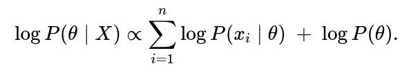
MAP, or Maximum A Posteriori, includes a prior term
P(θ)
and maximizes the posterior

. In log form, this becomes:

Hence, MAP differs by factoring in a prior. If the prior is uniform, MAP is equivalent to MLE.
Comprehensive Explanation
Conceptual Understanding of MLE
Maximum Likelihood Estimation (MLE) is a classical, frequentist approach. It seeks the parameter
θ
that maximizes the likelihood of observing the data at hand. If we assume observations

are independent and identically distributed (i.i.d.) under some model parameterized by
θ
, then the likelihood function is:

In practice, we often take the natural logarithm (log-likelihood) to transform the product into a sum:

Since the natural log is a strictly increasing function, maximizing the log-likelihood gives the same

as maximizing the original likelihood. This helps avoid potential numerical underflow issues (especially if the probabilities are very small) and simplifies derivatives for optimization.
Conceptual Understanding of MAP
Maximum A Posteriori (MAP) estimation is a Bayesian approach. Instead of only focusing on the likelihood, MAP incorporates a prior distribution
P(θ)
that encodes any pre-existing beliefs about the parameter
θ
before we see data. According to Bayes’ rule:

Because
P(X)
is a constant with respect to
θ
maximizing the posterior
P(θ∣X)
is equivalent to maximizing the numerator:

Switching to the log domain:
Hence, MAP estimation finds:

Key Difference
In MLE, we only optimize the likelihood term. In MAP, we optimize the sum of the likelihood term and the log-prior term. Whenever the prior
P(θ)
is uniform,
logP(θ)
is constant (does not depend on
θ
), so MAP simplifies to MLE.
Practical Motivations
MLE works well when the dataset is large and we do not have strong prior knowledge about the parameters. Because the likelihood is derived purely from observed data, it tends to converge to “reasonable” estimates if the sample size is big enough.
MAP is beneficial when we have prior beliefs about
θ
or if the dataset is small. Incorporating a prior can lead to more stable or better-controlled parameter estimates. For example, if we have a small dataset but prior knowledge thatθ
should be small, a prior favoring small values can shift the posterior accordingly, preventing overfitting or extreme estimates.
Potential Implementation Details
In machine learning libraries like PyTorch or TensorFlow, MLE often appears in forms such as maximizing the log-likelihood (for instance, with cross-entropy loss in classification). MAP can be implemented similarly, but with an additional regularization term that corresponds to the negative log of the prior. In practice, L2 regularization can be viewed as placing a Gaussian prior on parameters, while L1 regularization can be viewed as a Laplace prior.
For example, a basic PyTorch snippet illustrating MLE under a Gaussian assumption with unknown mean could look like:
import torch

# Suppose we have a dataset X with shape [n_samples]
X = torch.tensor([...], dtype=torch.float)

# We treat mean as a parameter, assume fixed variance
mean = torch.randn(1, requires_grad=True)

optimizer = torch.optim.SGD([mean], lr=0.01)

for epoch in range(1000):
    optimizer.zero_grad()
    # Negative log-likelihood for a Gaussian with mean=mean and var=1
    loss = 0.5 * torch.sum((X - mean)**2)  # This corresponds to -log P(X|mean)
    loss.backward()
    optimizer.step()

print("Estimated mean:", mean.item())
This code effectively performs MLE, because we are minimizing the negative log-likelihood (in this case, proportional to the squared error).
To turn this into a MAP estimation scenario with a Gaussian prior on
mean
(centered at zero, variance =

for instance), we would add a regularization term:
import torch

mean = torch.randn(1, requires_grad=True)
prior_variance = 1.0
optimizer = torch.optim.SGD([mean], lr=0.01)

for epoch in range(1000):
    optimizer.zero_grad()
    # Negative log-likelihood for Gaussian w.r.t. data
    data_term = 0.5 * torch.sum((X - mean)**2)
    # Negative log of a Gaussian prior ~ 0.5*(mean^2 / prior_variance)
    prior_term = 0.5 * (mean**2 / prior_variance)
    loss = data_term + prior_term
    loss.backward()
    optimizer.step()

print("Estimated mean with MAP:", mean.item())
Here, the prior_term corresponds to
−logP(θ)
under a Gaussian prior. This effectively biases the parameter to be near 0, which is typical of L2 regularization.
Possible Follow-Up Questions
What happens to MLE and MAP when the dataset size is very large?
When you have a very large dataset, the influence of the prior in MAP tends to get “washed out,” since the likelihood term usually dominates with a lot of data. Thus, MAP and MLE solutions often converge to very similar values. Practically, with huge datasets, the benefit of an informative prior is usually overshadowed by the massive quantity of available evidence in the data.
Why might we prefer MAP over MLE if the dataset is small or we have specific prior knowledge?
With small datasets, the likelihood alone might not provide enough information to robustly estimate parameters. If we have meaningful prior knowledge, MAP ensures that knowledge influences the final estimate. For instance, if you have prior reason to believe that a parameter should be sparse or close to zero, using an appropriate prior (like a Laplace prior for sparsity or a Gaussian prior for smaller absolute values) can guide the parameter estimation to remain near that region. This is particularly helpful to avoid overfitting when data is limited.
Can MAP be seen purely as adding a regularization term?
Yes, many regularization techniques in machine learning correspond to choosing particular priors in a Bayesian framework. L2 regularization can be viewed as a Gaussian prior on the parameters. L1 regularization can be seen as a Laplace prior. More complex priors (e.g., spike-and-slab) can lead to more advanced regularizers, but in essence, MAP is maximum-likelihood plus a prior-based term.
Is MLE a special case of MAP?
Yes, MLE is indeed a special case of MAP where the prior
P(θ)
is uniform over the parameter space. Because a uniform prior is a constant with respect to
θ
, it does not change the location of the maximum. Hence,

How do I decide whether to apply MLE or MAP in practice?
The choice often depends on:
Data Availability: If you have abundant data and little meaningful prior knowledge, MLE is simpler.
Prior Expertise: If there is genuine domain knowledge about
θ
, MAP is advantageous because it encodes prior beliefs.
Regularization Needs: In many practical machine learning tasks, we add a penalty term (like L2 or L1). This is essentially MAP with a corresponding prior. If overfitting is a concern, MAP (regularized approach) is typically preferred.
Could MAP estimates be more biased?
Yes, if the prior is strong but not reflective of reality, MAP estimates can indeed be more biased than MLE. However, in many real-world scenarios, using a correctly chosen or even moderately well-chosen prior can reduce variance and can improve predictive performance compared to an unbiased but higher-variance MLE estimate, especially in small-sample settings.
How does one select a prior for MAP?
Selecting a prior depends on domain knowledge, mathematical convenience, or both. Common choices:
Gaussian prior: Encourages smaller magnitude of parameters (L2 penalty).
Laplace prior: Encourages sparsity in parameters (L1 penalty).
Beta prior: Typical for parameters in the range [0,1], e.g., Bernoulli or binomial models.
Dirichlet prior: Generalization of Beta to multiple categories (common in topic modeling with LDA).
Choosing a prior typically involves examining the nature of the parameter and the distribution one expects it to have. In research settings, cross-validation or empirical Bayes methods may help refine prior hyperparameters.
Does MAP always produce a single parameter value?
Yes, in its basic form, MAP gives you a point estimate: the parameter value that maximizes the posterior. A fully Bayesian treatment, in contrast, would derive a posterior distribution over parameters rather than a single best estimate. MAP is effectively a middle ground between full Bayesian inference (which might integrate over the entire posterior) and the frequentist approach (MLE), where no explicit prior is assumed.
In what scenarios might MLE fail?
MLE can fail or be problematic when:
The likelihood function is poorly scaled or unbounded (e.g., certain unbounded distributions).
There is extreme multicollinearity or insufficient data (leading to very large variance in the estimate).
The model is too flexible (overfitting), in which case MLE might chase noise in the data.
MAP helps mitigate some of these by including prior information, acting like a regularizer.
Are there cases where MAP might be harder to implement than MLE?
Yes, because MAP requires specifying (and possibly integrating over) a prior, which can complicate optimization if the prior is complex or if the posterior is difficult to compute. MLE problems often turn into a straightforward optimization of the likelihood, which is simpler in some cases. Meanwhile, MAP can force you to handle additional hyperparameters (e.g., variance of your Gaussian prior) and tuning those can be nontrivial.
Below are additional follow-up questions
How do MLE and MAP handle missing data in a dataset, and what are the potential pitfalls?
When data is missing, neither MLE nor MAP can be directly applied to the incomplete dataset without modification. Typically, practitioners use methods like Expectation-Maximization (EM) to handle missing data:
For MLE: EM iterates between estimating the missing values (or their expected sufficient statistics) given the current parameter estimates (E-step) and maximizing the likelihood with respect to the parameters (M-step).
For MAP: EM can be adapted to incorporate priors, leading to a “Maximum A Posteriori” variant of the EM algorithm. The M-step would then maximize the posterior instead of the likelihood.
Potential pitfalls:
Non-ignorable missingness: If data are not missing at random (i.e., the missingness depends on unobserved variables or on the parameter itself), both MLE and MAP can produce biased estimates if the model does not account for the missing-data mechanism.
Local optima: EM (or MAP-EM) may converge to a local maximum, especially for complex models (e.g., mixture models). Proper initialization or multiple restarts might be necessary.
Overfitting if data is limited: With a large proportion of missing data, pure MLE might overfit. MAP, with a well-chosen prior, can regularize but might also be overly influenced by that prior if the dataset is very sparse.
What happens if the prior in MAP is misspecified or contradicts the observed data?
A prior can be misspecified either by being too restrictive (e.g., specifying a narrow range of parameter values that excludes the true parameter) or by failing to capture important characteristics of the parameter’s distribution.
If the prior is too strong: The posterior might be dominated by the prior, skewing the estimate and preventing the likelihood from effectively capturing the real data-generating process.
If the prior is too weak or diffuse: It becomes closer to uniform, which effectively reduces MAP to MLE. This might be acceptable, but it also defeats the purpose of having a prior if you truly have domain knowledge you want to incorporate.
Pitfalls:
False Confidence: A poorly chosen but strong prior can lead to very narrow posterior distributions that do not reflect reality.
Ignoring Contradictory Data: When the observed data strongly contradicts the prior, the posterior may still land in an incorrect region if the prior’s strength is set too high.
Partial data conflict: In some real-world settings, the data might partially agree with the prior but deviate in certain regimes. This partial mismatch can lead to subtle biases in the estimated parameters, often revealed only by extensive model checking or cross-validation.
In scenarios with complex or non-conjugate priors, how do we practically find MAP estimates?
When the posterior cannot be expressed in closed form or does not allow for direct maximization, practitioners resort to:
Numerical optimization: Use gradient-based methods (e.g., gradient descent, quasi-Newton methods) on the log-posterior. Frameworks like PyTorch, TensorFlow, or JAX can automatically compute gradients via backpropagation.
Approximate Bayesian inference: While MAP is not a fully Bayesian approach, techniques like Variational Inference or Markov Chain Monte Carlo (MCMC) can be adapted to locate high-density regions of the posterior, effectively approximating MAP solutions.
Pitfalls:
Multiple local maxima: Non-conjugate priors often result in posterior surfaces with many local maxima, requiring multiple initializations or specialized global optimization strategies.
High-dimensionality: As the parameter space grows, gradient-based methods may suffer from slow convergence or instabilities (e.g., vanishing/exploding gradients).
Choice of hyperparameters: Complex priors often bring additional hyperparameters (e.g., shape/scale parameters). If these hyperparameters are chosen poorly or not tuned, MAP estimates can be arbitrarily skewed.
Does MLE or MAP provide better predictive performance when the model is mis-specified?
Model mis-specification means that the true data-generating process is not accurately captured by the chosen model form (e.g., an incorrect family of distributions, missing interaction terms, etc.).
MLE: Can still fit the parameters that best align with the data under the incorrect assumptions, but may overfit or systematically deviate in certain regions.
MAP: The prior can help regularize the model, potentially mitigating some forms of mis-specification by preventing extreme parameter values. However, if the prior also aligns poorly with reality, MAP will not necessarily do better.
Pitfalls:
Bias-variance trade-off: MAP might reduce variance through regularization (prior), sometimes leading to better predictive performance even if the model is somewhat wrong. However, if the prior is invalid, the result can be both biased and suboptimal.
Overconfidence: A strongly regularizing prior might yield narrower prediction intervals, giving a false sense of certainty in predictions.
How do MLE and MAP approaches differ in mixture models, and what issues commonly arise?
Mixture models (e.g., Gaussian Mixture Models) involve latent variables indicating which mixture component generated each data point. Both MLE and MAP frequently use EM-based procedures:
MLE in Mixture Models: Focuses on maximizing the likelihood of the observed data, often leading to issues like overfitting, “label-switching” (identifiability), and convergence to spurious local maxima.
MAP in Mixture Models: Incorporates a prior on mixture weights, component means, and covariances. This can help avoid degenerate solutions (e.g., a component collapsing around a single data point with very small variance), because the prior penalizes extremely tight or trivial clusters.
Pitfalls:
Local Optima: Mixture models are notorious for local maxima in the likelihood/posterior. MAP does not eliminate this; it can still get stuck if the posterior has multiple modes.
Identifiability: Even with MAP, the labeling of mixture components remains ambiguous (“label switching”), requiring post-processing to match clusters across runs.
Unbalanced Clusters: If the prior strongly favors equal component weights, it might force an unrealistic distribution of cluster sizes.
What if we need interval estimates or measures of uncertainty in parameters for MLE and MAP?
MLE: Often uses asymptotic approximations. For large sample sizes, the distribution of the MLE around the true parameter can be approximated by a normal distribution with variance given by the inverse Fisher information.
MAP: You can approximate uncertainty by examining the curvature of the log-posterior around the MAP estimate (the Laplace approximation). However, MAP only gives a point estimate itself.
Pitfalls:
Small sample sizes: The asymptotic normal approximation for MLE can be inaccurate when data is limited.
Non-Gaussian Posteriors: MAP-based Laplace approximations can be very poor when the true posterior is multi-modal or highly skewed.
Ignoring systematic biases: Even if you get an uncertainty range, it may not capture model mis-specification or prior misalignment with the data.
What are practical considerations for setting the hyperparameters of the prior in MAP?
Hyperparameters govern the shape, location, or scale of the prior. For instance, in a Gaussian prior for weights in a regression, the variance parameter determines how strongly weights are shrunk towards zero.
Cross-validation: One of the most common ways to select hyperparameters is through a grid search or random search based on validation set performance or cross-validation error.
Empirical Bayes: Sometimes we estimate hyperparameters directly from the data by maximizing the marginal likelihood (though this can be computationally intense).
Domain knowledge: If domain expertise is available, it can guide the choice of hyperparameter values (e.g., typical effect sizes).
Pitfalls:
Overfitting to the validation set: If you tune too many hyperparameters or tune them too aggressively, you might overfit the validation.
Ignoring correlation among hyperparameters: In more complex priors, multiple hyperparameters may interact in complicated ways.
Computational overhead: Repeatedly optimizing a model with various hyperparameter settings can be computationally expensive, especially for large-scale models or big data.
How does regularization strength in MAP relate to Bayesian concepts?
In MAP with a Gaussian prior (L2 regularization), the variance of the Gaussian prior is inversely related to the regularization strength. A small variance prior means you strongly believe that parameters should be near zero, leading to heavier regularization.
Interpretation: In a simple regression with weights
w
, L2 penalty

corresponds to a prior on
w
that is Gaussian with variance
1/λ
Balancing data vs. prior: The ratio of the log-likelihood to log-prior gradient effectively determines how “trusting” you are of data relative to the prior.

Pitfalls:
Over-regularization: Setting regularization too high (equivalently, choosing a too-small prior variance) can overshrink parameters and degrade performance on complex tasks.
Under-regularization: A too-large prior variance (i.e., small or zero regularization) can lead to overfitting if data is limited.
Mismatch in parameter scales: If some parameters are expected to vary on vastly different scales, a single global regularization parameter might not be sufficient.
How do numerical optimization issues differ between MLE and MAP?
MLE: Usually requires optimizing

If this function is smooth and concave (or at least has a single global maximum in simpler models), gradient-based methods can converge reliably.
MAP: Involves


The additional term might introduce new curvature or complexity in the objective.
Pitfalls:
Non-smooth priors: A Laplace prior (L1 regularization) leads to absolute value terms in the objective, which are not differentiable at zero. Specialized optimization (like coordinate descent or subgradient methods) is needed.
Exploding or Vanishing Gradients: If the prior or likelihood is very sharp, gradient magnitudes can become extremely large or extremely small, complicating the optimization.
Ill-conditioned Hessian: Large or highly correlated parameter spaces can yield an ill-conditioned Hessian matrix for the log-posterior or log-likelihood, slowing down convergence or causing instability.
When might MAP produce pathological solutions, and how can we detect them?
“Pathological solutions” refer to unexpected or degenerate parameter values, such as extremely large or small estimates that do not make sense:
Under certain priors: A prior might concentrate mass on unrealistic regions. For instance, if it heavily favors extremely small variance in a Gaussian mixture, the algorithm might converge to near-zero variance for one cluster, ignoring the rest of the data.
In multi-modal posteriors: MAP might pick a spurious local maximum. The posterior could have a global maximum in a region that the algorithm never explores due to poor initialization.
Detection:
Check parameter magnitudes: If you see extremely large or tiny parameter values, it might indicate a pathological mode.
Use multiple starts: Optimize MAP from various initializations; if results differ drastically, you likely have multiple modes.
Monitor posterior predictive checks: Generate predictions from the MAP parameters. If they fail to resemble the actual data distribution, the solution might be pathological.