ML Interview Q Series: Modeling Server Wait Times Using a Mixture of Exponential Distributions

Browse all the Probability Interview Questions here.

15. Dropbox has just started and there are two servers for users: a faster server and a slower server. A user is routed randomly to either server. The wait time on each server is exponentially distributed but with different parameters. What is the probability density of a random user's waiting time?

Understanding The Question

The user is routed with probability 1/2 to the faster server and 1/2 to the slower server. Because each server’s wait time follows an exponential distribution, the resulting overall distribution is a mixture of exponentials. This means that the final probability distribution is the weighted sum of the two exponential pdfs, with weights equal to the probabilities of being routed to each server.

Core Concept: Mixture of Exponentials

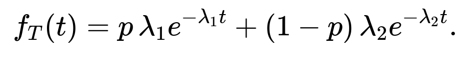
An exponential distribution with rate parameter λ has the pdf:

This function describes the probability density of the waiting time a random user experiences when the user is routed with 50% chance to either the faster or the slower server.

Detailed Reasoning and Explanation

• Because routing is random with equal probability, we form a 50–50 mixture of these two distributions. Mixture distributions arise frequently in queuing theory and practical load-balancing scenarios.

• The resulting pdf does not remain strictly exponential because it is a linear combination of two different exponential pdfs. It loses the memoryless property that a single exponential distribution has, because if you discover you are in a “slower” server route, the distribution of your waiting time is different from if you are in the “faster” server route.

• However, from a user’s perspective, all that matters is which server they happened to land on. If we look at the entire population of users without distinguishing which server they got, we must use this mixture pdf.

Final Probability Density

This is the direct and complete answer to the question.

Example Code Snippet for Generating Samples

Below is a short Python example illustrating how one might sample from this mixture distribution for simulation or testing. The code uses random choices to select which server rate is used, then samples from the corresponding exponential distribution:

import numpy as np

def sample_mixture_exponential(n_samples, lambda_1, lambda_2):
    # n_samples: number of samples to generate
    # lambda_1 : rate parameter for faster server
    # lambda_2 : rate parameter for slower server

    # Step 1: Decide which server gets picked for each user
    # with 50% probability each
    server_choices = np.random.choice(
        [1, 2],
        size=n_samples,
        p=[0.5, 0.5]
    )

    # Step 2: Generate the waiting times
    # For each choice, sample from the corresponding exponential
    wait_times = np.zeros(n_samples)
    mask_server1 = (server_choices == 1)
    mask_server2 = (server_choices == 2)

    wait_times[mask_server1] = np.random.exponential(1.0 / lambda_1, size=np.sum(mask_server1))
    wait_times[mask_server2] = np.random.exponential(1.0 / lambda_2, size=np.sum(mask_server2))

    return wait_times

# Example usage:
samples = sample_mixture_exponential(n_samples=100000, lambda_1=5.0, lambda_2=1.0)
print(np.mean(samples))

Practical Relevance

In the real world, especially in load balancing and cloud infrastructure, one often encounters mixtures of exponential (or other) distributions. Understanding that the overall waiting time can be modeled by a mixture helps in calculating average performance, tail probabilities, and other critical metrics for service-level agreements.

Possible Edge Cases and Subtleties

What if the servers receive different proportions of traffic rather than exactly 50–50?

Even though the original question implies equal probability routing, an interesting extension is to allow a fraction p to be routed to the faster server and 1−p to the slower server. The resulting pdf is then:

All the reasoning remains the same, but with different mixture weights. This can happen in practice if a load balancer is trying to shift more traffic to the faster server.

How does the memoryless property get affected in a mixture distribution?

The memoryless property of an exponential distribution states that, for an exponential random variable X with rate λ,

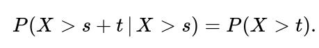
When we have a mixture of exponential distributions, the overall random variable does not generally maintain that memoryless property. Once you know you have “survived” a certain amount of time (say s), it changes the posterior probability that you are being served by the slower or faster server. Thus, a mixture of two distinct exponentials is not memoryless.

Why is this mixture distribution important in load-balancing scenarios?

In many real-world systems, not all servers are homogeneous. If you direct incoming requests randomly across machines of varying performance, each machine can be modeled with its own exponential service time parameter (assuming exponential service times). The overall distribution of service times across all machines (if a request can land on any machine) becomes a mixture. Practitioners need to know that mixture distributions behave differently than a single exponential, influencing average waiting times, throughput, and system reliability.

Yes. One practical approach would be:

• If logs do not specify the server, it becomes more complex since we only see the mixture distribution. In that case, one might use an Expectation-Maximization (EM) algorithm for fitting a mixture of exponentials to the data.

What if the question asked about the cumulative distribution function (CDF)?

You could find the mixture CDF by taking the weighted sum of each server’s exponential CDF:

How might we derive the moment-generating function (MGF) or characteristic function of a mixture?

For a mixture distribution, the MGF (moment-generating function) is the weighted sum of the MGFs of each component. For an exponential with rate λ, the MGF is:

Hence for the mixture:

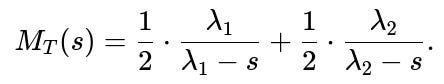
This can be used to find moments (like mean and variance) of T.

Could this distribution be generalized to more than two servers?

What are some tricky points an interviewer might emphasize here?

• Recognizing that the overall distribution is a mixture of exponentials, rather than a single exponential. • Understanding memoryless vs. non-memoryless properties. • Knowing how to compute the pdf, CDF, MGF, or other statistics from a mixture. • Understanding how to handle or estimate mixture parameters in practice. • A potential trick could be the ratio of usage if it’s not 50–50, or if the question tries to see if you mistakenly average the rates rather than forming the correct mixture pdf.

All of these details showcase an in-depth grasp of the subject, which is often tested in high-level machine learning or data science interviews that delve into statistics, probability theory, and the mathematics underlying real-world system performance.

Below are additional follow-up questions

What if the arrival process is not purely random, but follows a specific pattern like round-robin or time-based routing?

One might initially assume that when the question says "a user is routed randomly," it aligns with a memoryless arrival and assignment process. However, if users are routed in a round-robin fashion or according to any non-random scheme, the overall waiting time distribution might deviate significantly from a simple mixture of exponentials. In round-robin routing, each server receives requests in a specific sequence (for example, first user goes to Server 1, second user goes to Server 2, third user goes back to Server 1, and so on). This deterministic assignment can concentrate bursts of users onto each server in turn and might result in subtle correlations between consecutive arrivals and the state of each server. These correlations can undermine the assumption that each user’s waiting time is simply an exponential draw from one or the other server.

Pitfalls and edge cases: • If arrival rates are high, a server could build up a queue of waiting jobs, and because the routing is round-robin rather than random, the waiting times might grow in a pattern (periodic bursts) that a pure mixture model fails to capture. • In real systems with dynamic load conditions, a short run of heavy traffic might all be assigned to the same server before switching to the other server, altering the wait distribution from a neat exponential mixture. • If someone naively attempts to fit an exponential mixture to these waiting times, they might arrive at misleading parameter estimates because the data do not reflect independent random assignments.

How do we handle potential hardware failures, where a server becomes unavailable or temporarily overloaded?

In practice, one cannot always assume both servers remain operational with stable rates. If the slower server fails for a certain duration, the routing might redirect 100% of users to the faster server. Alternatively, if the faster server is not available, the system temporarily routes everyone to the slower server. This downtime or partial capacity changes the observed wait-time distribution.

Pitfalls and edge cases: • If a server goes down intermittently, the mixture proportions can shift drastically over time, invalidating the assumption of a fixed probability for each server. • Overloaded servers can effectively slow their service rates, so the actual rate parameter may drift outside the initially modeled range (for example, a server that was "faster" might slow to a crawl if it is overloaded). • Capturing these events might require time-varying mixture distributions or even a phase-type model. Real-world logs would show that the distribution of waiting times changes whenever a server experiences downtime or severe overload.

What if the service times on each server are not perfectly exponential, but follow a heavier-tailed or more complex distribution?

The assumption of exponential waiting times is often a simplifying one, rooted in the memoryless property. Yet, many empirical measurements in real systems show heavier tails (e.g., lognormal, Pareto) due to caching effects, bursty requests, or user behavior patterns. If each server’s waiting time distribution is not purely exponential, using a mixture of exponentials may be too simplistic.

Pitfalls and edge cases: • A mismatch between real data (which might have outliers or long tails) and an exponential mixture could produce systematically biased estimates for average wait times or tail probabilities (e.g., 95th or 99th percentile latencies). • The memoryless assumption might lead to underestimation of queue buildup under heavy load, whereas heavier-tailed distributions can cause long queues to form more frequently. • A robust approach might involve fitting a mixture of lognormal distributions or another parametric form that accommodates heavier tails.

What if we are interested in the distribution of waiting times conditional on the wait time already exceeding a certain threshold?

In practice, one might care about metrics like: “Given that a user has already waited 5 seconds, how much longer can they expect to wait?” With a single exponential distribution, the answer is straightforward due to the memoryless property. However, with a mixture of two different exponentials, the distribution is no longer memoryless. The conditional wait distribution would shift because the likelihood that the user is on the slower server increases if they have already been waiting.

Pitfalls and edge cases: • Failing to account for the non-memoryless nature of a mixture distribution can lead to incorrect predictions of how much longer a user might wait past a certain threshold. • Implementation decisions—such as reassigning a user to a different server after a certain wait—become more complex because you need to model the mixture dynamic properly. • In simulation or queueing analysis, one must condition on the event that the wait already exceeded a certain time, which might require Markov chain or Bayesian approaches to track the likelihood of being in the slow vs. fast server route.

How do we ensure the mixture rates and proportions remain consistent under scaling scenarios, such as adding more servers over time?

If the system scales up from two servers to many servers, the mixture model might evolve. For instance, one might add a third server that is even faster, or replicate the existing faster server to handle more load. Over time, the distribution of wait times would shift from a two-component mixture to a three- (or more) component mixture. This continuous change in infrastructure can make a static two-component model outdated.

Pitfalls and edge cases: • Relying on a fixed two-exponential mixture to analyze waiting times, while the real system keeps adding or removing servers, leads to inaccuracies in capacity planning. • The likelihood of capturing new states (such as an even faster server) can significantly change the overall waiting-time statistics, making it necessary to retrain or refit the mixture model frequently. • If one server receives a different fraction of traffic or has dynamic load balancing rules, the effective mixture weights might shift as the system grows, so historical data might not reflect current conditions.

Could a priority or reservation system skew the observed mixture distribution?

In some real-world systems, certain high-priority jobs or premium users get queued on the faster server preferentially. If a portion of traffic is always assigned to the faster server, the actual routing probabilities might not be uniform. This yields a conditional probability that is different from the naive 50–50 assumption.

Pitfalls and edge cases: • A priority queue might direct high-priority tasks to the faster server, leaving only low-priority tasks in the slower server’s queue. The resulting data could mislead an analyst trying to estimate a simple 50–50 mixture. • Mixed priorities within each server could still be described by an exponential distribution, but the routing logic complicates the mixture proportions. • The fraction of tasks that go to each server might not remain static over time (e.g., surges in premium usage), and a single stationary mixture model might no longer hold.

How would we implement real-time estimation of the mixture distribution parameters when logs only show wait times, not which server they came from?

Sometimes, logs only contain a user’s wait time without identifying the particular server that provided service. In that case, we only see the mixture distribution directly. To infer the mixture rates and weights in real time, one might attempt an online learning or streaming approach to fit the mixture of exponentials.

Pitfalls and edge cases: • Estimating mixture parameters from unlabeled data typically requires the Expectation-Maximization (EM) algorithm or a Bayesian approach. This can be computationally intensive for large-scale systems. • Online parameter updates might become unstable if the system’s load conditions or server performance changes frequently, causing the parameter estimates to fluctuate. • If multiple servers end up having very similar rates, numerical estimation can become ill-conditioned, making it difficult to distinguish between them in the mixture model.

What if we need to model not only the waiting time but also the server’s response time distribution under concurrency constraints?

If each server can serve multiple users simultaneously (with a maximum concurrency limit), the waiting time for each user depends on how many others are being served at that moment. This can lead to service time interactions that are no longer described well by a pure exponential for each individual user.

Pitfalls and edge cases: • Under concurrency, the effective service rate can diminish when many users share the same server, so the exponential parameter might change dynamically. • The question might pivot from “What is the distribution of a single user’s wait?” to “How do I model queue lengths or response times under concurrency limits?” which typically involves more elaborate queueing theory (e.g., Erlang or M/M/c queues). • If concurrency is high, a small difference in server capabilities might be overshadowed by concurrency effects, making the mixture distribution an oversimplification that misses the queue length buildup.

What if the question asks about the long-run steady-state distribution of waiting times in a queueing system?

So far, we mostly discussed the distribution of service times when a user is directly routed to an idle server. However, if both servers can develop queues, the waiting time distribution must account for how requests queue up over time. The result can be more complex than a simple mixture of exponentials, especially if arrival rates approach the sum of the servers’ capacities.

Pitfalls and edge cases: • In a stable queueing system (arrival rate below total service rate), the steady-state waiting time distribution might be derived using queueing theory like M/M/2 or some variant, which is not just a simple mixture of exponentials. • If traffic is high enough to saturate the servers, the system may not have a stable steady state, causing the average queue length to grow unbounded. • Real systems might use extra load balancing strategies (e.g., shortest queue routing), which changes the waiting time distribution dramatically compared to random routing.

How can we detect from real-world data that the mixture assumption might be invalid?

Sometimes a mixture of two exponentials is a good theoretical model, but actual logs or metrics might show discrepancies. One could compare the empirical distribution of wait times with the theoretical mixture distribution using techniques like the Kolmogorov–Smirnov test or Q-Q plots.

Pitfalls and edge cases: • A significant deviation between empirical data and the fitted mixture distribution might signal that the system is not truly a simple two-rate process (e.g., capacity constraints, concurrency, partial failures, or user behavior changes could all distort the distribution). • If the data exhibit too many long waits (heavy tail), then an exponential mixture might underpredict rare but extremely large values, suggesting a better fit with generalized Pareto or lognormal distributions. • Overfitting can occur if the system is dynamic and the user tries to fit a single mixture model to data that spans different operational regimes (peak vs. off-peak).

In practical monitoring and alerting, how can we leverage the mixture model for real-time decision-making?

Even if a mixture of exponentials is a rough approximation, it can still provide quick estimates of average wait times or tail latencies. Operators might use these estimates to set alert thresholds or auto-scaling triggers. However, they must be aware that a mixture model is only as accurate as its parameters and assumptions.

Pitfalls and edge cases: • If the system unexpectedly shifts from one operational mode to another (e.g., a major traffic surge), the previously calibrated mixture rates no longer match reality, causing incorrect alerts or missed alerts. • Overreliance on the average wait time, as opposed to the tail distributions, can hide service-level violations that occur under bursty conditions. • Real-time recalibration might be needed to track changes in server performance, so the mixture model does not become stale.

How do correlated arrival bursts impact the validity of the mixture distribution assumption?

In many real systems, users do not arrive independently; there may be sudden spikes in traffic (e.g., during peak hours or special events). If multiple users arrive nearly simultaneously, each server might receive a burst of requests. The mixture distribution alone cannot capture the subsequent queue buildup if the system was modeled only as “one user, one exponential wait.”

Pitfalls and edge cases: • Correlation in arrivals means the system can quickly shift from low utilization to very high utilization, affecting the distribution of waiting times in ways that a simple mixture model may fail to capture. • If the burst happens to route too many users to the slower server in a short time frame, observed waiting times can become skewed, leading to heavy right tails. • In real-world analytics, special care is needed to segment or cluster traffic by time of arrival so that bursty intervals do not contaminate the assumption of a stable mixture distribution.