
ML Interview Q Series: Modeling Uncertain Lifetime Spare Part Demand with Poisson Mixtures.

Browse all the Probability Interview Questions here.
A G–50 airplane is at the end of its lifetime. The remaining operational lifetime of the plane can be 3, 4, or 5 years, each with probability 1/3. A decision must be made about how many spare parts (denoted by Q) of a certain component to produce. The demand for these spare parts in each year of the plane’s remaining lifetime is Poisson-distributed with an expected value λ units per year, and the demands in different years are independent. Define X as the total demand for spare parts over the plane’s remaining lifetime.
What is the probability that the production size Q will not be enough to cover the total demand X (i.e., P(X > Q))?
What is the expected value of the shortage, that is E( (X − Q)⁺ ), where (x)⁺ = max(x, 0)?
What is the expected value of the number of units left over at the end of the operational lifetime of the plane, that is E( (Q − X)⁺ )?
Short Compact solution
Since the plane’s remaining lifetime can be 3, 4, or 5 years with equal probability 1/3, and demand each year is Poisson(λ), it follows that the total demand X is a mixture of Poisson distributions with means 3λ, 4λ, or 5λ. Concretely,
X has probability mass function given by (1/3) * [Poisson(3λ) + Poisson(4λ) + Poisson(5λ)], meaning P(X = k) = (1/3) ∑ from l=3 to 5 [ e^(−λl) (λl)^(k) / k! ].
The probability that Q units will not be enough is:
The expected number of spare parts left over is:
Comprehensive Explanation
Understanding how to calculate these probabilities and expectations requires carefully using the fact that a sum of independent Poisson random variables is itself Poisson, and that here, the total remaining lifetime of the plane is uncertain, with three equally likely possibilities.
Distribution of Total Demand X
Because each year’s demand is Poisson(λ) and there are l remaining years (where l can be 3, 4, or 5, each with probability 1/3), the total demand over l years is Poisson(lλ). Thus, the random variable X is a mixture (or compound distribution) of Poisson(3λ), Poisson(4λ), and Poisson(5λ). Specifically, with probability 1/3, the plane has 3 more years (so total demand is Poisson(3λ)), with probability 1/3, it has 4 years (Poisson(4λ)), and with probability 1/3, it has 5 years (Poisson(5λ)).
Hence, for k ≥ 0:
P(X = k) = (1/3) [ e^(−3λ) (3λ)^k / k! + e^(−4λ) (4λ)^k / k! + e^(−5λ) (5λ)^k / k! ].
Probability That Demand Exceeds Q
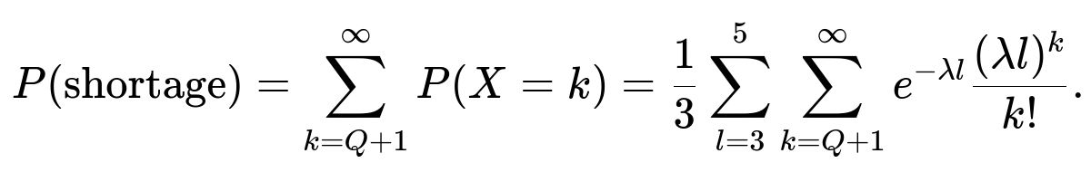
The event that the production quantity Q is not enough is (X > Q). We sum the above probability for k = Q+1 to ∞:
P(X > Q) = ∑ from k=Q+1 to ∞ P(X = k).
By plugging in the mixture form, we obtain:
(1/3) ∑ from l=3 to 5 [ ∑ from k=Q+1 to ∞ e^(−λl) (λl)^k / k! ].
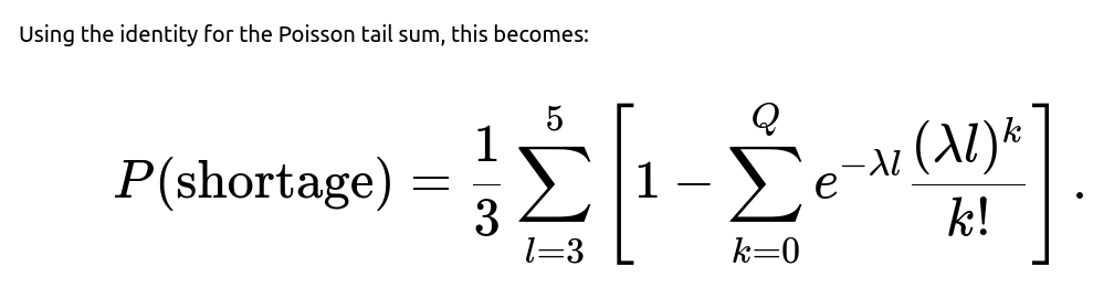
One can rewrite the Poisson tail probability ∑ from k=Q+1 to ∞ (λl)^k / k! e^(−λl) as 1 − ∑ from k=0 to Q e^(−λl) (λl)^k / k!. This yields the closed-form expression:
P(X > Q) = (1/3) ∑ from l=3 to 5 [ 1 − ∑ from k=0 to Q e^(−λl) (λl)^k / k! ].
Expected Number of Leftover Parts
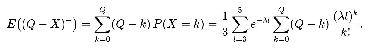
Define the leftover at the end of the plane’s life as (Q − X)⁺, which is zero if X exceeds Q or else Q−X if the demand is at most Q. Its expectation is:
E((Q − X)⁺) = ∑ from k=0 to Q (Q − k) P(X = k).
We substitute the mixture distribution for P(X = k), which gives:
E((Q − X)⁺) = (1/3) ∑ from l=3 to 5 [ e^(−λl) ∑ from k=0 to Q (Q − k) (λl)^k / k! ].
Expected Shortage
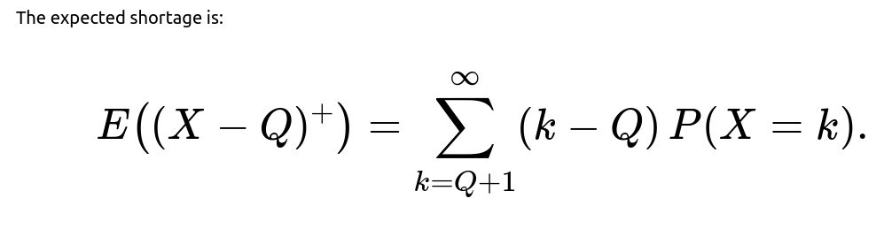
The shortage is (X − Q)⁺ = max(X−Q, 0). Its expectation is:
E((X − Q)⁺) = ∑ from k=Q+1 to ∞ (k − Q) P(X = k).
One can also use the fact that E(X) = 1/3(3λ + 4λ + 5λ) = 4λ for this mixture. A common way to see a relationship is:
(X − Q)⁺ = X − Q − (Q − X)⁺,
as long as we interpret it properly in expectation terms. After carefully summing over k≥Q+1 and rearranging terms, the expression becomes:
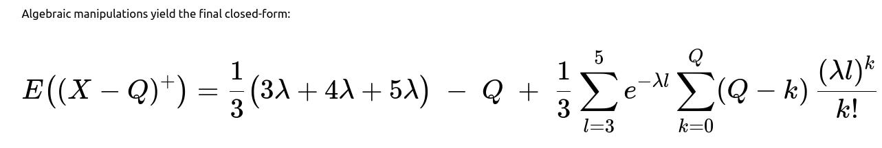
E((X − Q)⁺) = (1/3)(3λ + 4λ + 5λ) − Q + (1/3) ∑ from l=3 to 5 [ e^(−λl) ∑ from k=0 to Q (Q − k) (λl)^k / k! ].
This final expression highlights that the expected shortage is the difference between the plane’s average total demand (4λ) and Q, plus a correction term coming from how often and by how much Q exceeds actual demand.
Potential Follow-up Questions
Why is X a Mixture of Poisson(3λ), Poisson(4λ), and Poisson(5λ) Rather Than a Single Poisson Distribution?
Because the remaining lifetime l is itself uncertain (3, 4, or 5 years with probability 1/3 each). Conditional on l, the total demand is Poisson(lλ). If the value of l were fixed, X would simply be Poisson(lλ). However, since l is random, we must weight the conditional distribution by the probability of each possible l. This gives a mixture distribution, sometimes also called a “compound distribution,” which is an average of Poisson(3λ), Poisson(4λ), and Poisson(5λ).
Could We Have Computed E((X − Q)⁺) and E((Q − X)⁺) Without Summation Formulas?
Yes. One way is to use identities involving expectations of truncated random variables. For example, E((X − Q)⁺) can be linked to E(X) − Q − E((Q − X)⁺). However, eventually, one still needs to evaluate the needed probabilities of X ≤ Q or X > Q for the mixture distribution. For practical numeric purposes, people often just sum up the Poisson probabilities for k up to Q or from Q+1 to ∞.
How Would We Implement These Calculations in Python?
A straightforward approach is to compute each mixture component using built-in Poisson functions from libraries like scipy.stats.poisson. One could do something like:
import math
from math import exp, factorial
import numpy as np

def poisson_pmf(k, mean):
    return exp(-mean) * (mean**k) / math.factorial(k)

def shortage_probability(Q, lambd):
    # This calculates P(X>Q) using the mixture approach
    total_prob = 0.0
    for l in [3, 4, 5]:
        # Poisson(lambd*l)
        # sum_{k=Q+1 to inf} e^{-lambd*l} * (lambd*l)^k / k!
        # We can do 1 - sum_{k=0 to Q} pmf
        sum_up_to_Q = sum(poisson_pmf(k, lambd*l) for k in range(Q+1))
        total_prob += (1 - sum_up_to_Q)/3.0
    return total_prob

def expected_leftover(Q, lambd):
    # E((Q-X)+)
    leftover = 0.0
    for l in [3, 4, 5]:
        for k in range(Q+1):
            leftover += (Q - k)*poisson_pmf(k, lambd*l)/3.0
    return leftover

def expected_shortage(Q, lambd):
    # E((X-Q)+)
    # sum_{k=Q+1} (k - Q)*P(X=k)
    # or use the closed form expression from the solution
    # direct summation:
    short_val = 0.0
    for l in [3, 4, 5]:
        for k in range(Q+1, 200): # or some large cutoff
            short_val += (k - Q)*poisson_pmf(k, lambd*l)/3.0
    return short_val
One might truncate the sum at some large value (e.g., 200 or more) for practical numerical purposes. Alternatively, one can compute the exact tail sums using the identity for the Poisson distribution tail to make it more efficient.
Why Does E(X) = 4λ?
Taking l to be 3, 4, or 5 with probability 1/3 each, the expected value of l is (3+4+5)/3 = 4. Therefore the expected demand, being lλ, is 4λ overall.
What Happens in Extreme Cases?
If Q = 0 (making no spare parts), then the probability of shortage is obviously 1 − P(X=0), the expected shortage becomes E(X), and the leftover is 0. If Q → ∞ (making a very large supply), the probability of shortage approaches 0, the expected shortage goes to 0, and the leftover grows to E(Q−X) which approximately equals Q − E(X) in large Q limits, ignoring small tail probabilities.
How Does This Tie into Inventory or “Newsboy” Models?
This is a form of the classic single-period or multi-period inventory model, except that the “periods” are uncertain in total length. One might optimize Q by balancing costs of shortage versus leftover, leading to a standard newsvendor-type solution. The difference here is that the total demand distribution is a mixture of Poisson distributions rather than a single known distribution.
All these considerations are crucial in a real-world setting, especially if the cost of leftover parts or the penalty for shortage is large. Interviewers often check if candidates understand both the conceptual derivation and the computational aspects (e.g., using tail sums for Poisson or numerical approximations) as well as the potential use of such results in making practical decisions (e.g., finding an optimal Q).
Below are additional follow-up questions
How does uncertainty in λ across the years affect the model?
In many practical situations, the demand rate λ might not be constant across years. It could fluctuate based on changes in usage patterns, maintenance schedules, or the operational context of the plane (e.g., a plane might fly more hours in its last year if it’s being leased elsewhere). If λ is uncertain and can vary from year to year, then the total demand distribution may no longer be a simple Poisson(lλ) even conditionally on l. Instead, you might need a more general compound-Poisson or mixed-Poisson model where each year i has its own λi. Specifically, if l=3, the demand would be Poisson(λ1+λ2+λ3), provided these λi are known. However, if λi themselves are random and correlated, the model complexity increases.
Edge case concerns:
Parametric uncertainty: You might not know λ1, λ2, λ3 precisely, which calls for Bayesian methods where λi are random variables with certain priors.
Time-varying rates: If λi are systematically increasing or decreasing each year (e.g., usage is ramping up), ignoring that can bias your estimates.
Non-Poisson arrival processes: Real demands may exhibit seasonality or correlation between consecutive years, potentially invalidating the simple Poisson assumption in some domains.
A more robust approach might be to model each year’s demand with its own distribution (possibly Poisson with separate parameters or a negative binomial if overdispersion is observed). You then aggregate them accordingly, still weighted by the probability that l=3,4, or 5.
How would we handle salvage value for leftover parts?
In classic inventory or newsvendor problems, leftover items may have a nonzero salvage value. For instance, if leftover parts can be sold back to a supplier or repurposed for another airplane model, then producing extra spares isn’t a total loss. This modifies the objective function for choosing Q, because leftover items mitigate the penalty of overestimating demand.
Potential pitfalls:
Partial salvage: If the salvage value is partial, the leftover cost is not simply Q−X but includes some salvage offset. In that case, E((Q−X)⁺) is replaced by a cost-based function that accounts for the net of holding cost minus salvage revenue.
Unexpected changes in salvage: If the resale market price is volatile, the salvage value might be uncertain. One might need to incorporate a probability distribution or scenario-based approach for salvage value.
Contractual constraints: Some components cannot be resold due to regulatory or safety reasons, so salvage might be zero in such a scenario.
What if the random variable l is not equally likely to be 3, 4, or 5?
The question scenario assumes each of 3, 4, and 5 years is equally likely, but in reality, the probabilities might differ. For instance, if historical data shows that planes of this type typically retire after 3 years 50% of the time, 4 years 30% of the time, and 5 years 20% of the time, you would change the mixture weights accordingly.
Implications:
The mixture distribution becomes P(X=k) = p3 * Poisson(3λ) + p4 * Poisson(4λ) + p5 * Poisson(5λ), where p3+p4+p5=1.
The expected number of years is now 3p3 + 4p4 + 5p5, and hence the average demand is λ(3p3 + 4p4 + 5p5).
If these probabilities p3, p4, p5 are poorly estimated, your inventory decisions might be systematically biased.
Pitfalls:
Misestimation of l: If l is often overestimated, you risk producing too many spares. If l is underestimated, you risk shortages.
Continuous distribution of lifetimes: In practice, the plane might not have discrete possibilities of 3, 4, or 5 years but a more continuous range (e.g., anywhere between 3 and 5.5 years). You then need a distribution for l and integrate over that distribution.
How do correlated demands between years affect the calculations?
The standard assumption is that each year’s demand is independent. However, in some real-world settings, if one year has unusually high usage, it might carry over into the following year due to increased wear and tear or the aging nature of certain parts.
Consequences:
The sum of correlated Poisson demands is generally not Poisson. This complicates the distribution of X. Instead, one might approximate the total demand via a compound distribution or use moment-based approximations (e.g., negative binomial, gamma-Poisson mixtures).
Probability of shortage calculations are more complex; straightforward formulas for Poisson tail sums no longer apply.
Simulation-based approaches (Monte Carlo) can become more practical if the correlation structure is well-defined.
Pitfalls:
Mis-specified correlation structure: If the correlation is incorrectly estimated, predictions of extreme demands may be off.
Increased variance: Correlation typically increases the variance of the total demand, raising the chance of shortage if Q is chosen under an independence assumption.
What if the plane’s demand changes partway through its remaining lifetime?
Sometimes, the usage pattern or the maintenance routine for the airplane could change drastically after, say, 1 year. This might happen if the plane is sold to a new airline with different flight schedules. In that case, you don’t have a uniform Poisson(λ) demand each year; perhaps the first year is λ1 and subsequent years are λ2.
Pitfalls:
Piecewise-defined distribution: If the plane has 3 remaining years but changes usage after year 1, you have a Poisson(λ1) demand for the first year and Poisson(λ2) for the next 2 years. Summation rules still hold, but the total demand for 3 years becomes Poisson(λ1+2λ2), complicating the mixture with other lifetimes.
Non-stationary demand: Demand rates may ramp up or down, so a single parameter λ per year may not suffice.
Can we incorporate lead time for producing additional spare parts?
In practice, one might not have to set Q just once. There could be a possibility of restocking if the plane’s lifespan extends or if the demand is higher than expected. However, if producing new spares takes time (lead time), shortages might still occur temporarily.
Key points:
Multi-stage inventory: If you can reorder mid-lifetime, the problem becomes a dynamic inventory control problem rather than a one-shot decision. This changes the entire modeling approach (e.g., dynamic programming or multi-period newsvendor).
Lead time vs. lifetime: If the plane’s lifetime is short, lead time might be comparable to the entire horizon, rendering reorders impractical.
Demand forecasting update: After observing one or two years of actual demand, you might update your belief about λ and adjust Q accordingly.
What numerical stability issues might arise during implementation?
When computing Poisson probabilities, one might have to calculate terms like (λl)^k / k!, which can become numerically unstable for large k. Also, exponentials e^(−λl) can underflow for large λl.
Potential solutions and pitfalls:
Logarithmic computations: Instead of directly computing e^(−λl) (λl)^k / k!, it’s often safer to use log-probabilities to avoid floating-point underflow.
Recursive relations: Poisson pmf can be computed via a recursion: P(X=k+1) = (λl/(k+1)) P(X=k). This reduces reliance on factorial and large powers.
Cutoff for tail sums: When summing tails up to ∞, you typically truncate at some large k (like k=200 or more) if λl is moderately sized. You must ensure the tail is negligible or else use a function that can compute Poisson tail probabilities directly for better precision.
How would you choose an optimal Q in practice?
One might want to minimize a cost function that balances the shortage penalty with the leftover cost or salvage value. The typical approach is the “newsvendor formula,” but modified for the mixture distribution of X.
Steps:
Define a cost function: cost(Q) = shortage_cost * E((X−Q)⁺) + holding_cost * E((Q−X)⁺).
Plug in the mixture distribution for X.
Solve for the Q that minimizes cost(Q). Because Q is discrete, you might have to search over integers or use an iterative approach.
Compare with a continuous approximation to get an initial guess.
Pitfalls:
Exact integer optimization: If Q is large, searching all possible Q can be computationally expensive. One might rely on approximate or iterative methods.
Uncertain cost parameters: If shortage cost is difficult to estimate (e.g., how much does a grounded plane cost per day?), it becomes tricky to choose Q accurately.
Risk preferences: If management is extremely risk-averse, they might choose a Q that’s higher than the standard cost-minimizing solution.