ML Interview Q Series: Navigating Non-i.i.d. Data: Statistical Techniques for Time-Series and Grouped Data Challenges.

📚 Browse the full ML Interview series here.

i.i.d. Assumption: What does it mean to assume that data points are *i.i.d.* (independent and identically distributed)? Why is this assumption important for many statistical machine learning methods, and what issues can arise if your dataset violates the i.i.d. assumption (for example, in time-series or grouped data)?

Definition of the i.i.d. Assumption

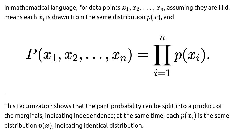
The idea of independent and identically distributed (i.i.d.) data points is fundamental in statistical machine learning. Independence means that each data point does not inform or constrain any other data point in your dataset. Identically distributed means that all data points are drawn from the same underlying probability distribution. When both of these conditions hold, we say that the dataset is i.i.d.

Significance of the i.i.d. Assumption in Statistical and Machine Learning Methods

Many foundational results in statistics and machine learning rely on the i.i.d. assumption:

Convergence guarantees for methods such as gradient-based optimization in neural networks. The derivation of the loss function as an average of independent samples typically presupposes i.i.d. data. Statistical consistency theorems for estimators such as the Maximum Likelihood Estimator or the Empirical Risk Minimization principle assume independence. These theorems often require that data is sampled from the same distribution. Generalization bounds, such as the Probably Approximately Correct (PAC) framework, typically assume the training and test data come from the same distribution and that each sample is independent of the others. Validation and test strategies (e.g., cross-validation) assume that each split of the dataset is representative of the same underlying distribution. Independence helps ensure that random splits produce unbiased estimates of performance.

When the i.i.d. assumption is violated, many classical theoretical guarantees—like unbiasedness, consistency, and generalization bounds—might no longer hold, or they become much harder to prove or interpret.

Issues That Arise When the i.i.d. Assumption is Violated

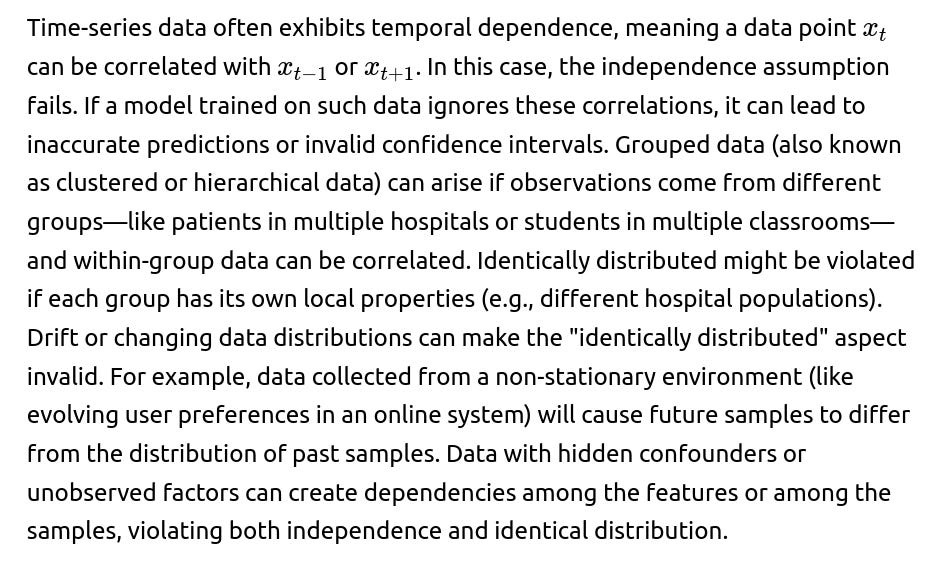
Real-World Examples and Practical Implications

In time-series forecasting, you have an inherent structure where each observation is correlated with the past. Standard i.i.d. methods might fail to capture autocorrelation patterns. Instead, specialized time-series models (e.g., ARIMA, LSTM-based sequence models) or data transformations (e.g., differencing) are used to respect the temporal structure. In recommendation systems, user data can come in sessions or be influenced by multiple contextual factors. Treating sessions as i.i.d. samples can obscure vital temporal and contextual dependencies. Grouped or hierarchical modeling can help here, such as using multi-level models that incorporate group-level random effects. In large-scale observational studies—like health records from various hospitals—data from each hospital can differ in subtle ways, violating identical distribution. Adjusting for hospital-level effects or domain adaptation can help mitigate these distribution differences.

Handling Non-i.i.d. Data in Practice

When facing non-i.i.d. data, one can adopt methods designed for those structures:

Time-series analysis with models that capture dependencies across time (e.g., RNNs, LSTMs, Transformers with sequence modeling, or classical ARIMA and state-space models). Mixed-effects or hierarchical models for grouped data, which introduce random effects to capture group-level variations that break the identical distribution assumption. Block bootstrap or specialized cross-validation strategies (e.g., time-series cross-validation) for correct estimation of model performance. Domain adaptation and transfer learning methods for data drift or distribution shifts, ensuring the model can adapt to changes over time.

Code Example Illustrating Proper Handling of Time-Series Cross Validation

Below is a simplified snippet of Python code using scikit-learn-like pseudo-structures to show how to handle time-series splits properly, acknowledging the serial dependence in data:

import numpy as np
from sklearn.model_selection import TimeSeriesSplit
from sklearn.linear_model import LinearRegression

# Synthetic time-series data
np.random.seed(42)
time_series_length = 100
X = np.arange(time_series_length).reshape(-1, 1).astype(float)
y = 2 * X.squeeze() + np.random.normal(scale=5, size=time_series_length)

model = LinearRegression()
tscv = TimeSeriesSplit(n_splits=5)

for train_index, test_index in tscv.split(X):
    X_train, X_test = X[train_index], X[test_index]
    y_train, y_test = y[train_index], y[test_index]

    model.fit(X_train, y_train)
    score = model.score(X_test, y_test)
    print("Train indices:", train_index, "Test indices:", test_index, "R^2:", score)

In this example, we use a TimeSeriesSplit that respects the temporal ordering, preventing data leakage from the future into the training set. This highlights how to adapt cross-validation when the i.i.d. assumption is violated by time-order dependencies.

How might you test whether data violates the i.i.d. assumption?

One can examine correlation structures. For time-series data, autocorrelation plots or partial autocorrelation plots can reveal significant correlations over lags. If data is grouped, you can check whether the distribution of features or the target is similar across different groups. Major discrepancies could indicate violation of the identical distribution assumption. Formal statistical tests, such as the Durbin-Watson test for serial correlation in regression residuals, or other tests for stationarity in time series, can also help identify violations.

How do we adjust our modeling strategy if data is not i.i.d.?

When data is dependent across time, incorporate lags or sequence models (e.g., ARIMA, RNN, LSTM, Transformers). When data is grouped, adopt hierarchical models or random effects. When data shifts over time, use online learning or domain adaptation to update the model with incoming data. When data is high-dimensional and potentially correlated, regularization or structured sparsity can help capture the underlying dependence structure.

What if we still apply i.i.d.-based methods to non-i.i.d. data?

Performance metrics might be overly optimistic because the evaluation strategy might ignore the dependencies. Confidence intervals or hypothesis tests might be invalid. The derived p-values and intervals could drastically misrepresent true uncertainty. Generalization can degrade in practice because the assumption that training and test data come from the same distribution (and that samples are independent) is violated.

In practical ML pipelines, how to detect and correct i.i.d. violations early?

Exploratory Data Analysis (EDA) focusing on time or group variables to see if data is stable over time or across groups. Tracking metrics in production systems to detect concept drift (e.g., if a model’s performance degrades over time, that may suggest that distribution has changed). Introducing data versioning and continuous monitoring of feature distributions to spot distribution shifts.

Why is the i.i.d. assumption essential for theoretical guarantees?

Most classical theorems, such as the Law of Large Numbers, Central Limit Theorem, and PAC learning bounds, rely on the idea that the variance in the sample mean decreases with more independent samples. If the samples are correlated or come from different distributions, deriving these results or bounding generalization error is significantly more complex or might require additional assumptions.

Could we partially relax the i.i.d. assumption without losing all theoretical backing?

Yes, there are theoretical frameworks for analyzing data that exhibit certain types of dependency:

Mixing processes in time series or Markov chain assumptions provide ways to extend theoretical results to dependent data if certain mixing coefficients remain small. In multi-task or grouped learning scenarios, specialized theoretical analyses can handle hierarchical structure. These approaches require more complex proofs but still yield approximate or weaker versions of classical results. Stationarity assumptions in time series can replace the requirement for identical distribution with the requirement that the underlying process statistics do not change over time.

Follow-up Questions

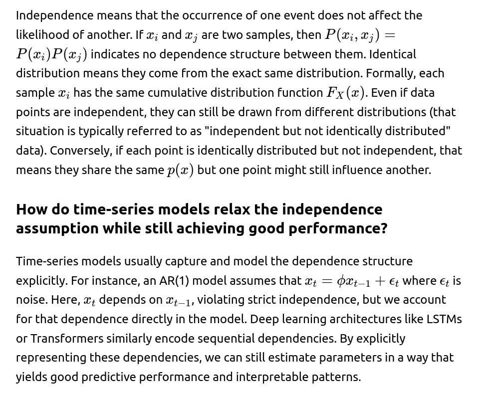
Could you explain the difference between "independence" and "identical distribution" in more depth?

What is the role of stationarity in time-series analysis?

Stationarity is the concept that statistical properties (like mean, variance, autocorrelation) do not change over time. Strict stationarity requires the joint distribution of a sequence of variables to be invariant to shifts in time. For many theoretical results in time-series analysis, some form of stationarity is assumed so that the behavior learned from past data applies consistently to future data. When stationarity is violated (e.g., in trending or seasonal data), transformations or specialized modeling (like differencing for ARIMA, or seasonal ARIMA) become necessary.

If we have grouped data (e.g., data from multiple cities), do we completely lose the i.i.d. assumption?

You do not necessarily lose it entirely, but you have to be cautious. Often, within each city, data might share group-level traits, so points in the same city might be more similar to each other than to points in another city. That breaks the global assumption that any two data points in the entire dataset are identically distributed and independent. A typical approach is hierarchical or multi-level modeling, where variation is captured at both the global level and the city-specific level. In this framework, you can still make strong inferences, but it involves modeling those dependencies and differences among groups explicitly.

Are there any specific pitfalls one must watch for when randomly splitting a dataset that violates i.i.d. assumptions?

If data is time-dependent and you randomly split training and test sets, data from the future can leak into the training set, causing artificially inflated performance metrics. If data is grouped, random splitting can cause partial data from a single group to be in both training and test sets, again overestimating real performance. The model might learn group-specific patterns that do not generalize well. It is safer to do group-wise splits (so all data from any single group is entirely in train or test) or time-series splits (training on early periods, testing on later ones).

How does concept drift in an online system violate the identical distribution assumption?

Concept drift means the data’s distribution changes over time (e.g., user preferences shift, external market factors change). This directly violates the assumption that each data point is drawn from the same distribution. A model trained on old data might no longer see the same distribution in the future. Methods to handle concept drift often involve incrementally retraining, weighting recent data more, or actively detecting points in time when the distribution changes.

How can you mitigate the violation of independence in data that arises from repeated measurements?

Repeated measurements of the same entity (e.g., the same patient measured multiple times) are correlated. Instead of ignoring this correlation, you can: Use random effects models: These treat repeated measurements within an entity as correlated through a shared random effect term. Use repeated measures ANOVA or equivalent time-series approaches: These can handle the correlation structure. Use cluster-robust standard errors in linear models if the correlation structure is not too complex.

What is the central limit theorem (CLT) for dependent data and how is it different from the classical CLT?

A CLT for dependent data typically requires the concept of weak dependence or mixing conditions. In these cases, the sample means might still converge to a normal distribution as the sample size grows, but the speed of convergence or the variance of the limit distribution can differ from the classical i.i.d. result. Classical CLT requires independence and identical distribution, so the expansion to dependent data demands additional conditions on how quickly the correlation in the sequence decays.

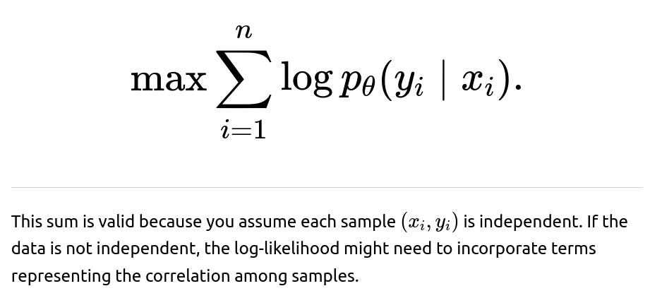
How does i.i.d. factor into the derivation of losses like cross-entropy or mean squared error?

Common training objectives are typically derived under the assumption that each data point is sampled from the same distribution and that the likelihood of observing the entire dataset is the product of each observation’s likelihood (the factorization property). For cross-entropy in classification, you are effectively maximizing the likelihood under the assumption:

What are practical steps for diagnosing if a machine learning model’s assumptions of independence are breaking?

Look at residuals for patterns over time or across groups. If there is structure left in the residuals, that often indicates dependence. Perform correlation tests among features or among samples. If you see strong correlation patterns for data points that are close in time or belong to the same group, that is a red flag. Compare performance from naive cross-validation to more carefully structured cross-validation (like time-series split or group-based split). If results differ drastically, you likely have a violation of the i.i.d. assumption.

How does batch normalization or dropout in neural networks relate to i.i.d. data assumptions?

Batch normalization uses statistics (mean, variance) computed from a batch of samples. In principle, it often assumes these mini-batches are representative of the overall distribution. Non-i.i.d. data within a batch can lead to misleading estimates of mean and variance. This is particularly problematic if the data is heavily time-dependent or if certain classes or groups are not well-represented in each batch. Dropout randomly drops units independently at each training step, which also presupposes that samples are somewhat independent. If data is heavily correlated, dropout might still help regularize the network, but we need to be cautious about how well that regularization addresses correlated structures.

How does the i.i.d. assumption tie into the VC dimension and capacity control?

When deriving bounds on the generalization error using VC dimension or Rademacher complexities, we rely on an assumption that each training example is drawn i.i.d. from a common distribution. This ensures that expected errors over the training sample can generalize to the population distribution. Violations of this assumption complicate or invalidate these bounds, making it harder to reason about a model’s capacity and overfitting risks.

Why might it still be helpful to approximate data as i.i.d. even if it’s not strictly true?

Many real-world datasets have mild dependencies or distribution shifts that might not completely break i.i.d. assumptions. Even if the data is not strictly i.i.d., the assumption might be a useful approximation—especially in high-level neural network training—if the violation is not extreme and specialized methods to model the dependencies are too complex. In practice, the i.i.d. assumption is often made by default because many algorithms and theories are built upon it. If the violation is modest, results can still be decent. If it is severe, ignoring it leads to errors, so that triggers the need for specialized modeling.

How does non-i.i.d. data interact with large language models (LLMs)?

Large language models like GPT variants are often trained on massive corpora that include correlated documents, repeated text segments, and shifting distributions over time (especially if the data covers many years or domains). Although the training data is not strictly i.i.d., the scale of the data often makes the assumption of i.i.d.-like random sampling from a giant pool a workable approximation in practice. However, in fine-tuning or domain adaptation contexts, it is crucial to be aware of distribution shifts (e.g., specializing a model to a narrower domain). If the newly introduced data is from a different distribution, domain adaptation or further fine-tuning is needed.

Is there a formal approach to quantifying how much a dataset deviates from i.i.d.?

One approach is to quantify correlation within subsets of the data or across time steps. Another is to measure distribution differences, such as using Kullback–Leibler divergence between data blocks over time or across different groups. The higher the divergence, the larger the violation of identical distribution. Advanced approaches might use metrics like Maximum Mean Discrepancy (MMD) to compare distribution similarity between subsets of data, or to compare training vs. test distributions.

What is a scenario where data is identically distributed but not independent?

Imagine you sample from the same distribution for every data point (so the distribution is identical), but for each pair of consecutive samples, there is some correlation structure. This can happen in processes like Markov chains with a fixed stationary distribution. Each sample is drawn from that same stationary distribution, but each sample’s value depends on the last. This is a common scenario in time-series, making them identically distributed under stationarity assumptions but not fully independent.

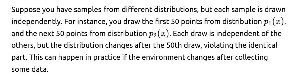
What is a scenario where data is independent but not identically distributed?

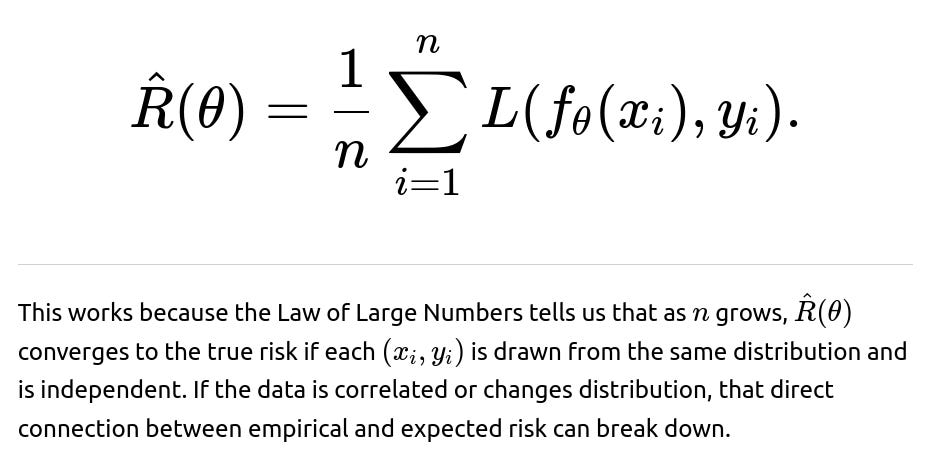
Why does the i.i.d. assumption enable simpler forms of risk estimation?

The expected risk under i.i.d. sampling can be estimated by the empirical risk using a simple average:

Could ensemble methods be used to address non-i.i.d. data?

Ensemble methods like bagging, boosting, or random forests typically assume that data is sampled i.i.d. from the same distribution, especially bagging which uses bootstrap samples. When the data is heavily time-dependent or has group structure, naive bagging might not solve the problem of correlation. However, if the i.i.d. violation is mild, ensembles can still help reduce variance and might partially mitigate some negative effects of the violation. For strong dependency or distribution shifts, specialized strategies (like time-series ensembles or grouped ensembles) are needed.

How do we adapt standard cross-validation for grouped data?

When you have grouped data, a typical method is group-aware cross-validation, ensuring that all data from a single group is included entirely in either training or test. In scikit-learn, there is a GroupKFold approach. For example:

import numpy as np
from sklearn.model_selection import GroupKFold
from sklearn.linear_model import LogisticRegression

X = np.random.rand(10, 3)
y = np.random.randint(2, size=10)
groups = np.array([1,1,2,2,3,3,4,4,5,5])  # group labels

group_kfold = GroupKFold(n_splits=5)
clf = LogisticRegression()

for train_index, test_index in group_kfold.split(X, y, groups=groups):
    X_train, X_test = X[train_index], X[test_index]
    y_train, y_test = y[train_index], y[test_index]
    clf.fit(X_train, y_train)
    score = clf.score(X_test, y_test)
    print("Train groups:", groups[train_index], "Test groups:", groups[test_index], "Score:", score)

This ensures that each group’s data is separated between training and test folds, reducing contamination from group-specific patterns.

When is ignoring the i.i.d. assumption still acceptable?

If the correlation or distribution shift is minor, ignoring i.i.d. might not drastically degrade performance, especially if you have a large dataset. If you do quick prototyping or proof-of-concept experiments, you might accept the i.i.d. assumption initially, while planning to refine your approach later for production use. If the domain or regulatory environment is not strict about statistical inference (like p-values or confidence intervals) and you primarily care about raw predictive accuracy, you might “get away” with ignoring mild violations.

Is the i.i.d. assumption more crucial in certain sub-fields of ML?

Fields like econometrics, biostatistics, or clinical trials often place strong emphasis on correct inference, standard errors, and p-values, so independence and identical distribution matter greatly. In purely predictive tasks (like large-scale recommendation systems), while i.i.d. assumptions are technically violated, large data and robust algorithms might handle mild violations relatively well, albeit with less clear theoretical guarantees.

How might one approach domain adaptation if the i.i.d. assumption fails due to distribution shift?

Domain adaptation involves methods such as re-weighting samples (important sampling in feature space), learning domain-invariant representations (adversarial domain adaptation), or fine-tuning a pre-trained model on a new domain. These methods aim to align or adjust the distributions between training and test (or source and target) domains to mitigate the violation of identical distribution.

How does the concept of exchangeability differ from i.i.d.?

Exchangeability means that any reordering of the sequence of random variables does not change the joint distribution. For i.i.d. data, the data is automatically exchangeable, but certain processes can be exchangeable without being strictly i.i.d. Exchangeability is a weaker condition than i.i.d., but still underpins some Bayesian approaches, like the De Finetti theorem for infinitely exchangeable sequences.

Why do so many text and image datasets approximate i.i.d. sampling?

When constructing datasets like ImageNet or large text corpora for natural language processing, the data is collected in a random manner from numerous sources. Each image or text snippet is often treated as an independent sample from a large pool. Although not strictly true, the heterogeneity and random sampling from a broad enough source often makes it a passable approximation.

How does reinforcement learning (RL) handle the lack of i.i.d. in state transitions?

In RL, data is generated by an agent interacting with an environment, causing strong temporal correlations between consecutive states. The typical i.i.d. assumption in supervised learning does not hold. RL methods use experience replay buffers, target networks, or on/off-policy learning to partially decorrelate samples or account for the Markov Decision Process structure. This is an explicit acknowledgment that data is not i.i.d.

How might we approach the final choice of data splitting or modeling when i.i.d. is questionable?

Always perform domain-specific checks. For time-series, do time-based splits. For grouped data, do group-based splits. If you detect distribution shifts, adapt your model (domain adaptation or continual learning). Validate your approach with error metrics that reflect real-world usage. For instance, if predicting future outcomes, ensure that your validation set indeed mimics the future scenario. Continuously monitor the performance in production. If performance degrades, investigate whether distribution shifts have become more pronounced.

Conclusion of Discussion

The i.i.d. assumption underlies a huge portion of statistical and machine learning theory and practice. It offers elegant derivations and generalization guarantees. However, when data exhibits temporal or group-wise dependence, or when distribution shifts over time, the i.i.d. assumption can fail—potentially invalidating naive modeling, training, and evaluation procedures. In such scenarios, specialized modeling or data-splitting techniques are necessary to maintain robust performance and reliable uncertainty estimates.

---

Below are additional follow-up questions

What are the potential implications of label distribution shift versus feature distribution shift on the i.i.d. assumption?

When people discuss violations of the i.i.d. assumption, they often focus on the idea that both features and labels might not be drawn from the same distribution in training versus test (or in different segments of the data). A subtle but important case is when the feature distribution remains largely consistent, but the label distribution shifts. For instance, imagine a spam detection system that sees a stable linguistic distribution of emails (features) over time, but the actual proportion of spam vs. not-spam (labels) changes drastically during holiday seasons. This scenario violates identical distribution on the label side, even if the feature side is unchanged.

In this situation, the classifier might become poorly calibrated. It will assume the likelihood of "spam" or "not spam" is the same as in the training phase and could produce more false positives or false negatives. Real-world pitfalls include:

• Calibration errors. If the decision threshold was tuned on a 50/50 spam-to-ham ratio, a shift to 70/30 would skew predictions badly.

• Class imbalance issues. As label proportions drift, the model might underperform for the minority class, especially if the minority class was significantly different during training.

• Over/under thresholding. The model might not adjust because it assumes the prior class probabilities do not change, potentially leading to mismatched expectations of false positive/false negative rates.

A robust approach includes continuously monitoring label proportions, periodically recalibrating threshold decisions, and using techniques like online learning that update probabilities as new labeled data becomes available.

How does the i.i.d. assumption play a role in online learning algorithms, and what if it’s violated?

Online learning setups typically assume new data points arrive sequentially, possibly drawn from the same distribution as previous samples (an i.i.d. assumption). Algorithms like stochastic gradient descent (SGD) rely on the idea that each new sample is an unbiased estimate of the true gradient.

When the i.i.d. assumption is violated in online settings:

• The step sizes might lead to divergence or poor convergence if the underlying distribution changes repeatedly (concept drift).

• The gradient updates may represent different underlying tasks or distributions, making classical convergence proofs invalid.

• The model might be forced to “forget” older data too quickly or too slowly, depending on how the distribution evolves.

Mitigations include:

• Using sliding window approaches where only recent data is used to update the model, accommodating potential drift.

• Incorporating adaptive learning rates or methods like ADAGRAD, RMSProp, or Adam, which can more flexibly handle changes in gradient magnitudes.

• Implementing drift detection systems that trigger partial or full model retraining once certain statistical tests indicate a shift.

Pitfalls or Edge Cases:

• If drift is abrupt (e.g., a total change in user behavior after a sudden event), a gradual adaptation mechanism might lag significantly.

• If drift is cyclical (like weekly user patterns), simply discarding older data might lose valuable information about repeated future cycles.

How do bootstrap or resampling methods rely on i.i.d. assumptions, and what happens if data is not i.i.d.?

Bootstrap methods create synthetic datasets by sampling with replacement from the original dataset to estimate variability or uncertainty (such as confidence intervals of a model). These techniques typically hinge on the idea that each data point in the original set is an independent draw from a common distribution.

If data is not i.i.d. (for example, time-series data with autocorrelation):

• The standard bootstrap would repeatedly sample points that are sequentially correlated, thus not reflecting the true distribution of the residuals or the actual random process over time.

• This can lead to overly optimistic or misleading confidence intervals. The variability captured might be smaller than the real-world variability.

Possible solutions:

• Use block bootstrapping in time-series contexts, where contiguous blocks of data are sampled to retain correlations.

• Use moving-block or stationary bootstrap if the correlation structure is complex.

• For grouped/clustered data, cluster bootstrap can be used to keep group correlations intact.

Potential Edge Cases:

• If correlation extends over long time horizons, even block bootstraps might fail unless blocks are appropriately sized.

• If data is heavily unbalanced in terms of groups, you could over- or under-sample certain groups repeatedly.

How can partial i.i.d. assumptions be applied if only subsets of the data meet those criteria?

In some situations, the entire dataset might not satisfy i.i.d. assumptions, but well-chosen subsets do. For example, a global e-commerce dataset might have strong differences between countries or regions. Within each region, the data might look more i.i.d. than the global set.

One strategy is to split the dataset according to the domain or grouping factor, ensuring each subset is closer to i.i.d. Then you can:

• Train a local model per subset if each subset is sufficiently large.

• Train a single global model but incorporate domain-specific features or domain-adaptation layers.

• Use hierarchical models that share parameters across subsets but allow local variations.

Potential pitfalls:

• Over-segmentation. If you create too many subsets, some subsets become too small to train robustly.

• Confounding differences. Even within subsets that seem consistent, hidden differences or distribution drift over time can still violate i.i.d. locally.

Is there a distinction between i.i.d. assumptions in supervised versus unsupervised learning?

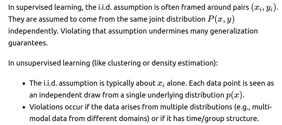
Edge Cases:

• In anomaly detection, data might be mostly i.i.d., but anomalies themselves might have different correlations or distributions.

• In generative modeling, if data is not identically distributed, the learned generative model might severely misrepresent minority subsets.

How do data augmentation techniques in deep learning relate to the i.i.d. assumption?

Data augmentation (e.g., random flips, rotations for images, or noise injection in text) is typically used to artificially expand a training set under the assumption that these augmentations do not change the underlying class distribution or introduce spurious correlations. The assumption is that an augmented sample is another valid i.i.d. draw from the same distribution.

But problems can arise:

• Overly aggressive or unrealistic augmentations can create training examples that do not exist in the real distribution (leading to distribution mismatch).

• Non-i.i.d. data with domain-specific constraints might not benefit from naive augmentations. For example, flipping medical images horizontally might invalidate anatomic references.

Pitfall Examples:

• In text augmentation, random word swaps might break linguistic dependencies or grammar, introducing samples that do not conform to real usage.

• Using the same augmentation random seed for all images in a mini-batch can create artificial correlations among the augmented samples.

How do labeling errors or noisy labels affect the i.i.d. assumption?

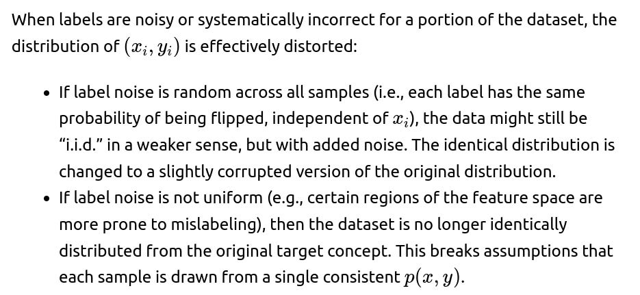
Edge Cases:

• Crowdsourced labeling where certain annotators might consistently label incorrectly or have a bias can create patterns in labeling noise that break independence.

• If data is sorted or grouped by labelers with different biases, you can have distribution shifts in labeling accuracy across data segments.

How does using synthetic or generative data for training intersect with i.i.d. assumptions?

Sometimes models are trained or partially trained on synthetic data generated by a simulator. The simulator might aim to replicate the real-world distribution, but rarely does it capture all complexities:

• If synthetic data distribution does not match the real data distribution, “identically distributed” is violated when you mix synthetic data with real data in training or testing.

• Overfitting to synthetic artifacts can cause poor real-world performance.

Edge Cases:

• Real data may have rare edge cases or anomalies the simulator never generated, causing the model to fail in real scenarios.

• Simulator-level correlation. If a simulator reuses certain procedural generation seeds or logic, it may produce correlated samples that are not truly independent.

How might the i.i.d. assumption break if training and deployment environments differ significantly?

A model may be trained in a controlled environment (like a lab) where data is carefully collected. At deployment, it faces real-world data that can deviate significantly:

• Changes in device sensors, or changes in user behavior, can lead to distribution shifts, breaking the assumption that test data is drawn from the same distribution as training data.

• Shifts in label definitions or feedback processes in the real world can also cause the model to encounter label distributions different from those seen during training.

Potential pitfalls:

• Model drift if the environment evolves too quickly or unpredictably.

• The system might fail silently if there is no continuous monitoring or feedback loop that captures the difference.

Can private or federated learning setups suffer from i.i.d. violations?

In federated learning, data remains on local client devices and the model is updated in a distributed fashion. Each client might have a unique data distribution, which can be different from other clients. This is called “non-IID” data in federated learning:

• Standard federated averaging algorithms assume each client’s local update is a fair sample of the global distribution. If each client has unique usage patterns, this assumption is violated.

• Convergence might be slower or might favor clients that have distributions closer to the average.

Edge Cases:

• Personalization is often introduced to mitigate major distribution mismatches. However, if distributions vary heavily, global model performance can degrade.

• Clients with very small datasets might produce high-variance gradient estimates, hurting global convergence.

Could we have a scenario where the data is i.i.d. in high-level aggregates but not in fine-grained structure?

Yes. For instance, daily sales data might appear to be i.i.d. day-by-day at the aggregate level. However, within each day, there is strong correlation (e.g., hourly patterns) that break independence. Summarizing at the day level can mask intra-day correlations but might appear i.i.d. at the daily resolution.

Pitfalls:

• Missing out on important sub-daily patterns, causing incomplete modeling.

• Overlooking cyclical or seasonal effects if the day is considered a single data point.

What approaches exist for quantifying the extent of non-i.i.d. structure in big datasets?

Some advanced techniques:

• Copula-based methods to measure dependencies among variables or among data points.

• Intrinsic dimension or manifold learning analysis to see if some data sub-manifolds share distribution properties distinctly from others.

• Bayesian hierarchical modeling, which explicitly encodes group and sub-group variations, can reveal the extent to which each group differs from a global distribution.

Pitfalls:

• High complexity of these methods can lead to overfitting or intractable computations in large datasets.

• Real-world data often has multiple overlapping forms of dependence (time + groups + hidden confounders), complicating any single measure of “non-i.i.d.”

How does the i.i.d. assumption affect interpretability methods like SHAP or LIME?

Many local interpretability methods assume that small perturbations of a single instance are reflective of realistic samples from the same distribution. If features are correlated or if the data distribution has complex dependencies:

• Perturbation-based methods might sample unrealistic or improbable feature combinations, leading to misleading local explanations.

• If part of the dataset is from a different distribution, an interpretation derived from one subset could be meaningless for another subset.

Edge Cases:

• Time-series features that must remain in consistent temporal order to make sense can be incorrectly permuted or perturbed.

• Categorical features with group structure: random perturbations that shuffle categories might produce nonsense samples (like mixing countries and cities incorrectly).

What unique challenges does active learning face when the data pool is not i.i.d.?

Active learning selects the most informative samples to label. The typical theoretical framework often assumes those selected samples come from an i.i.d. pool.

If the pool is not i.i.d.:

• The selection mechanism might focus on anomalies or interesting sub-regions that differ from the main data distribution. This can bias the model if it over-represents certain patterns.

• If new data arrives over time in a non-stationary manner, a static pool-based active learning approach may not adapt well.

Pitfalls:

• The model’s view of “informative” points might keep changing if the distribution evolves, leading to incomplete coverage of future domain changes.

• If data is grouped, the active learner might keep sampling from the same group it deems uncertain, ignoring other groups.

How do multi-armed bandit or contextual bandit settings address the non-i.i.d. nature of streaming data?

Bandit algorithms typically assume each reward sample (from pulling an arm or presenting an action) is independent. However, user preferences and contexts can be correlated over time, breaking independence.

For contextual bandits:

• The assumption is that each context-reward pair is drawn from a stationary distribution. In practice, user behavior evolves (non-stationary).

• Algorithms like EXP3 or Thompson Sampling might be robust to mild non-stationarity but can fail if major drift occurs.

Potential pitfalls:

• A bandit might “lock in” on a strategy that performs well initially but is suboptimal once user preferences change.

• If context features are heavily correlated (e.g., multiple contexts come from the same user in short succession), the reward estimates might become biased.

Does the i.i.d. assumption break when we do oversampling or undersampling for class imbalance?

Techniques like SMOTE or random oversampling artificially replicate minority class samples or synthesize new minority samples. This can violate independence if the new synthetic points are strongly influenced by existing minority points in the feature space. However, many practitioners still treat them as if they were new i.i.d. draws.

Potential pitfalls:

• Overfitting to the minority class, especially if oversampled points do not introduce genuinely new patterns.

• Underestimating real-world complexity if the minority class is not truly well-represented even after synthetic generation.

Are there scenarios where data is “conditionally i.i.d.” given certain latent variables?

Sometimes data can be viewed as i.i.d. if we condition on certain hidden or latent variables. For example, in a mixture model scenario, if the mixture component (latent variable) is known for each sample, then within each component, data might be i.i.d. from that component’s distribution. Without conditioning on the latent variable, the entire dataset appears non-i.i.d. from a single global perspective.

Pitfalls:

• Identifiability. You might not know the correct latent variables or might have too many/few components.

• Overly simplified latent structure. Real data might have more intricate dependencies than a finite mixture assumption can capture.

How might cross-correlation among features or among samples complicate the i.i.d. assumption?

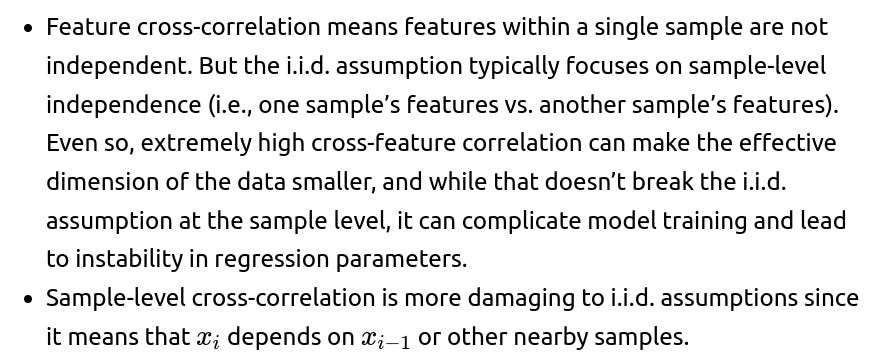
Edge cases:

• Data with repeated patterns or near-duplicates can create effectively correlated samples. This might artificially inflate model performance in a random split evaluation.

• Very high correlation among features can lead to numerical instability in matrix-based methods like OLS if not handled by regularization or dimensionality reduction.

Does the i.i.d. assumption hold in reinforcement learning when the reward function changes mid-deployment?

If the environment changes its reward function—say, a game’s rules are updated—this directly invalidates the assumption that reward samples come from the same underlying distribution. The agent’s previous experiences are from one distribution, while future experiences come from another.

Pitfalls:

• The policy might become suboptimal or worthless in the new environment without a mechanism for adaptation.

• The agent may exhibit catastrophic forgetting if it overfits to the new environment and discards all knowledge from the previous version, some of which might remain partially relevant.

In ensemble methods that use bagging, does non-i.i.d. data cause any special concerns beyond standard single-model approaches?

Bagging draws bootstrap samples from the original dataset to train multiple base learners. If the dataset is not i.i.d.:

• Re-sampling from correlated data might produce multiple bootstrap sets that are not representative. Instead of capturing random variation, each bootstrap might replicate correlated segments.

• This can lead to ensembles overestimating their own confidence because each base learner sees correlated patterns, reducing the overall variance they are supposed to capture.

Edge cases:

• Extremely correlated data (like multiple near-duplicate samples) can cause bagging to produce nearly identical models.

• If data has strong grouping, random sampling with replacement can break group structures, leading to artificially inflated performance in cross-validation.

How does the i.i.d. assumption shape the idea of permutations or randomization tests in hypothesis testing?

Randomization or permutation tests rely on the assumption that data points are exchangeable (a weaker condition than i.i.d. but closely related). If data has a known structure (e.g., chronological ordering or grouping), random permutations might break that structure, invalidating the test’s foundation.

Pitfalls:

• When time-series or grouped data is permuted, the test statistic distribution might not reflect reality, producing incorrect p-values.

• If a grouping factor is crucial, permutations that mix group labels can destroy within-group correlations, creating a mismatch with the real data-generating process.

What special considerations are needed for anomaly detection when the i.i.d. assumption does not hold?

In anomaly detection, a model is often trained to understand the “normal” data distribution. If data is i.i.d., outliers are easier to identify statistically. If data is correlated:

• A point could appear anomalous if viewed in isolation, but it might be perfectly normal in the context of a correlated sequence (e.g., a spike in time-series data that always follows a certain pattern).

• Non-stationary data might make certain points appear anomalous when in fact they represent a new normal.

Edge Cases:

• In streaming anomaly detection with concept drift, the definition of “normal” changes over time, requiring adaptive thresholds.

• Correlated anomalies (e.g., multiple sensors failing in a correlated manner) might lead to false negatives if the detection approach only searches for individually anomalous points without considering group correlations.

Can data imputation techniques inadvertently break or assume i.i.d. structure?

When imputing missing data, methods like mean imputation, k-nearest neighbors, or regression-based imputation often assume the observed data is representative of the same distribution from which the missing values originate. If the missingness mechanism depends on time or group factors, or if the dataset is not identically distributed across subsets:

• The imputed values might systematically bias the final dataset.

• Correlations might be introduced between samples if the same imputation model is used across different groups that truly differ.

Pitfalls:

• If missingness is not at random and is related to unobserved factors, standard imputation can severely distort relationships.

• Time-series data typically needs specialized imputation (e.g., forward filling, interpolation) that respects temporal order.

Does the i.i.d. assumption impact how we tune hyperparameters, for instance in Bayesian Optimization?

Bayesian Optimization typically treats each hyperparameter configuration’s performance as an independent sample from a latent function. If the data used to evaluate a model’s performance for one hyperparameter is correlated with the data used for another in subtle ways (like shared cross-validation folds that have temporal dependence), the assumption of independent noise in the objective function might fail.

Potential consequences:

• Over- or underestimating certain hyperparameter configurations.

• The GP (Gaussian Process) or surrogate model used in Bayesian Optimization might produce inaccurate uncertainty estimates if performance measurements are correlated in non-trivial ways.

Edge Cases:

• If the validation set changes distribution mid-optimization, some hyperparameters might look artificially strong or weak compared to earlier runs.

• If each iteration reuses the same non-i.i.d. data splits, performance evaluations might systematically favor certain configurations.

How might the i.i.d. assumption interact with data privacy constraints (like differential privacy)?

Differential privacy algorithms often add noise to data or model parameters to protect individual sample privacy. This process usually assumes that each sample’s contribution to the overall statistic is independent. If samples are correlated (for example, multiple records belonging to the same person), it can weaken the intended privacy guarantees because removing or changing one person’s data might not fully anonymize that person’s correlated records.

Pitfalls:

• Repeated correlated records can allow an adversary to pinpoint an individual even after the noise injection because the correlation boosts the signal of that individual’s data pattern.

• Group-level correlation can mean the privacy budget is consumed at a faster rate if many correlated records belong to the same individual or cluster.

How do you avoid incorrectly attributing poor model performance to hyperparameter tuning if i.i.d. is violated?

When i.i.d. is violated, some hyperparameters might appear suboptimal simply because the dataset splits do not reflect real-world usage. Steps to avoid confusion:

• Use domain-aware splitting methods (time-series splits, group splits) to measure performance more realistically.

• Track performance metrics over time or across groups to see if certain hyperparameter choices only fail in specific scenarios.

• Deploy smaller scale tests or pilot phases to confirm that any improvement during training is consistent in real usage conditions.

Edge Cases:

• Overfitting to a specific time window or group distribution might cause the chosen hyperparameters to fail in the next window or group.

• If distribution shifts quickly, repeated hyperparameter tuning might chase a moving target.

How does the i.i.d. assumption shape our interpretation of feature importance in a model?

Feature importance metrics, whether in linear models (coefficients) or tree-based models (split frequency, SHAP values), generally assume that the distribution of data used to estimate these metrics is representative of the true data distribution. If the data shifts or has subgroups with different relationships:

• Feature importance can be misleading or might average contradictory effects across subgroups.

• Time-varying feature importance might never be captured by a single global measure.

Edge Cases:

• A feature might appear very important globally but be useless for a new segment of data that changed distribution.

• If the dataset includes multiple correlated sub-populations, the feature importance might reflect only the largest sub-population’s relationships.

When deploying a model to new regions or customer segments, how can the i.i.d. assumption fail specifically?

Geographic or demographic expansion can introduce new feature distributions (e.g., different average income, cultural preferences) or new label distributions. The i.i.d. assumption that “new region data matches old region data distribution” breaks immediately. Common pitfalls:

• The model might underperform or fail catastrophically if crucial features shift in meaning (e.g., addresses or local norms).

• The evaluation metrics used during training do not reflect how the new region’s data will behave.

Mitigations:

• Gradually collect labeled data from the new region or segment to refine or retrain the model.

• Use transfer learning or domain adaptation to incorporate knowledge from the original domain while adjusting to local specifics.

How can cross-correlation among samples be exploited rather than simply lamented as a violation of i.i.d.?

While correlation among samples violates i.i.d. assumptions, it can also be a source of structure. Graph-based approaches, for example, explicitly model relationships among nodes (samples). In recommendation systems, user-user or item-item similarities are harnessed to improve predictions. In time-series, using memory-based models improves predictive power.

Pitfalls:

• Overfitting to spurious correlations if the model is too flexible and the correlation is ephemeral.

• Increased complexity in training and model building, requiring specialized frameworks (graph neural networks, Markov models, etc.).

Could external or exogenous factors break i.i.d. assumptions suddenly (e.g., a natural disaster or policy change)?

Yes. If something happens that drastically alters user behavior or data generation, your trained model might see data from a distribution it has never encountered. This goes beyond typical drift—it's a sudden distribution jump. Common pitfalls:

• The model might produce completely unreliable outputs in the aftermath of such an event.

• Historical data can become almost irrelevant for immediate predictions.

Possible responses:

• Rapid retraining using any available post-event data.

• Incorporating robust or scenario-based modeling that can simulate rare events.

What are recommended best practices for diagnosing and handling i.i.d. violations in a standard ML workflow?

• Perform thorough exploratory data analysis (EDA) with a focus on time-based or group-based stratifications.

• Choose appropriate splitting strategies: time-based or group-based cross-validation when relevant.

• Monitor distribution of features and labels over time to detect drift.

• Use specialized models or transformations (time-series, hierarchical, domain adaptation, etc.) instead of purely i.i.d.-based techniques.

• Validate results with domain experts who can confirm whether observed patterns are stable or context-dependent.

Pitfall:

• Ignoring warning signs like unusual changes in performance metrics across subpopulations.

• Relying solely on average performance metrics might mask serious issues in certain slices of the data.