ML Interview Q Series: Negative Hypergeometric: Probability of r-th Red Ball on the k-th Draw

Browse all the Probability Interview Questions here.

A bowl contains n red balls and m white balls. You randomly pick without replacement one ball at a time until you have r red balls. What is the probability that you need k draws?

Short Compact solution

Define E0 as the event that you get r - 1 red balls in the first k - 1 draws, and E1 as the event that the kth draw is a red ball. Then

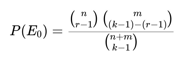
Here n is the total number of red balls, m is the total number of white balls, r is the target number of red balls we want to draw, and k is the total number of draws after which we have exactly r red balls.

Next,

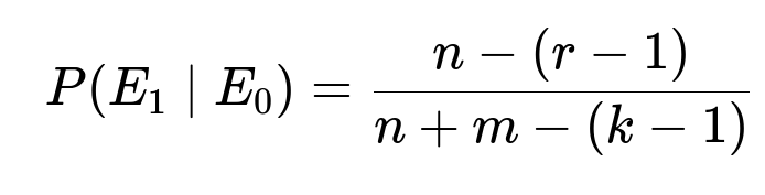
which is the probability that the kth ball is red given that we already have r - 1 red balls in the first k - 1 draws. Therefore, the desired probability is

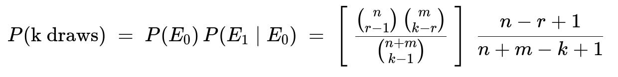
valid for k ranging from r up to m + r.

Comprehensive Explanation

Combinatorial reasoning

To find the probability that the rth red ball appears precisely on the kth draw, we look at two parts. First, we must ensure that in the first k - 1 draws, we have exactly r - 1 red balls. Second, on the kth draw, we get a red ball.

The number of ways to choose exactly r - 1 red balls out of n available red balls and (k - 1) - (r - 1) white balls out of m available white balls is given by the product of binomial coefficients binom(n, r - 1) and binom(m, (k - 1) - (r - 1)). These choices cover all possible ways to form a subset of k - 1 balls containing r - 1 reds and (k - r) whites. The total number of ways to choose any k - 1 balls from the n + m total balls is binom(n + m, k - 1). Hence P(E0) becomes that ratio of binomial coefficients.

Conditioning on E0, we know that there are n - (r - 1) red balls left in the unchosen portion of the bowl, and there are n + m - (k - 1) total balls remaining. So the probability that the kth ball is red (event E1) is the ratio (n - (r - 1)) / (n + m - (k - 1)). Multiplying P(E0) by P(E1 | E0) yields the probability that the rth red ball occurs on the kth draw.

Range of k

It only makes sense to achieve the rth red ball on draw k once k is at least r, because you cannot have r red balls in fewer than r draws. Furthermore, you cannot exceed k = m + r because in the worst case you could draw all m white balls before finally obtaining the rest of the red balls, which would mean you would achieve the rth red on the (m + r)th draw at the latest.

Relation to the Negative Hypergeometric Distribution

This distribution is a classic example of the negative hypergeometric distribution, which models the probability distribution of the draw on which the rth success (in this case, drawing a red ball) occurs when sampling without replacement.

Importance in Machine Learning contexts

Although the question might appear purely combinatorial, such reasoning often underpins advanced topics in ML and statistics where sampling without replacement appears, especially in importance sampling or in analyzing certain random partitioning schemes. Understanding how hypergeometric and negative hypergeometric probabilities behave is valuable for confidence intervals and bounding arguments in ML analysis.

Edge considerations

If r = 1, then the question reduces to the probability that the first ball is red, which obviously is n / (n + m). If r = n, one might wonder about the boundary scenario in which every red ball must be drawn. In that extreme, the last red ball might appear as late as n + m (if we somehow draw all white balls first). The formula still holds by substituting r = n.

Potential follow-up question: Derivation from first principles

One way to derive the distribution from scratch is to consider permutations of the n + m balls. In how many permutations does the rth red ball appear in the kth position? We can systematically count permutations that have r - 1 red balls in the first k - 1 positions, the kth position red, and the remaining n - r red balls distributed among the last (n + m - k) positions. This combinatorial argument directly yields the same formula. The advantage of first principles is that it clarifies why the distribution is called “negative hypergeometric”: it is about the trial count at which a certain cumulative threshold of red balls is reached.

Potential follow-up question: Connection to real-world problems

Many real-world processes involve sampling without replacement until a certain number of “marked” items are found. Examples include quality control (finding defective items in a batch) or searching for r relevant documents among a mixture of relevant and irrelevant ones. Understanding how to compute the probability distribution of the time (or number of draws) until the rth success arises frequently in such acceptance-sampling or retrieval tasks.

Potential follow-up question: Implementation in Python

A direct implementation of the probability can be done using Python. One may compute binomial coefficients via math.comb in Python 3.8+ or with scipy.special.comb. For instance:

import math

def negative_hypergeom_pmf(n, m, r, k):
    numerator = math.comb(n, r-1) * math.comb(m, (k-1) - (r-1))
    denominator = math.comb(n + m, k - 1)
    conditional = (n - (r - 1)) / (n + m - (k - 1))
    return (numerator / denominator) * conditional

# Usage example:
n = 5   # number of red balls
m = 7   # number of white balls
r = 3   # we want the 3rd red ball
k = 6   # the number of draws
prob = negative_hypergeom_pmf(n, m, r, k)
print(prob)

This code calculates the exact probability that the 3rd red ball appears on the 6th draw, given 5 total red and 7 total white balls.

Potential follow-up question: What if sampling was with replacement?

If we were sampling with replacement, each draw is an independent Bernoulli trial for drawing a red ball (with probability n/(n+m) of being red if we imagine n red and m white, but replaced every time). The distribution of the trial on which the rth success occurs would then be given by the Negative Binomial distribution, which has a different PMF. This distinction is critical in machine learning contexts (for instance, with bootstrapping, sampling might be considered with replacement; with cross-validation data splits, sampling is often without replacement). Hence, the subtle differences in the distribution highlight the importance of carefully verifying the assumptions about sampling strategies.

Potential follow-up question: Handling large values in practice

When n, m, and r are large, direct computation of binomial coefficients can become numerically challenging. It can be handled by either using floating-point logarithms of binomial coefficients or using stable functions such as scipy.special.loggamma in Python. Ensuring numerical stability can be essential when dealing with large sample sizes, which is often the case in data-intensive machine learning pipelines.

Below are additional follow-up questions

What happens if r exceeds the total number of red balls, i.e., r > n?

If r is greater than n, the event of drawing r red balls is impossible. Consequently, the probability of ever reaching r red balls in that scenario is zero. This might sound trivial, but in real-world data situations—especially when parameters are inferred from noisy measurements—it’s possible to plug in values that violate such constraints. Practitioners must ensure that r is always within [1, n] before applying the negative hypergeometric formula. If, for instance, data collection or parameter estimation erroneously suggests r > n, you would want to revisit your data-cleaning or parameter-estimation steps to make sure they align with physical or logical constraints of the problem.

How can we obtain the expected number of draws needed to get r red balls?

The negative hypergeometric distribution has a known mean (expected value) for the draw on which the rth red ball appears. In plain text, the expected value is (r * (m + n + 1)) / (n + 1). However, in actual practice you might want to derive or confirm it via summing k times the PMF over all k from r to r + m. That summation approach can be numerically large but is conceptually straightforward. From an interview perspective, knowing that a closed-form solution for the expectation exists shows that you grasp both the distribution and its key statistical properties. A subtle pitfall is relying on the distribution’s expectation as a single descriptor. If the distribution is highly skewed (for instance, if r is close to n, or if m is very large compared to n), then the variance can be substantial, and so “expectation alone” might be misleading for real-world scheduling or risk-analysis decisions.

Can we extend the negative hypergeometric setting to multiple categories (more than just red and white)?

Yes, the negative hypergeometric framework can be extended when there are more than two categories. However, the direct formula for “the draw on which the rth item of type A appears” becomes more complicated if there is also type B, type C, and so forth. One common approach is to collapse all the non-target categories (everything that is not red) into a single effective category, effectively returning to a two-category problem. This works only if we do not distinguish among the other categories individually. A subtlety arises if we need to keep track of partial counts of multiple different colors or categories. In that case, the distribution becomes a multivariate version of the hypergeometric family. For r = 1 and multiple categories, you can adapt negative hypergeometric arguments, but the combinatorial forms can become cumbersome. In practical ML or data-analysis tasks, it might be simpler to apply direct combinatorial or simulation-based methods.

Are normal or other large-sample approximations ever appropriate?

Yes, large-sample approximations can be used if n and m are both large. A normal approximation to the negative hypergeometric distribution might be invoked via a central limit theorem argument, especially when r is not too close to 0 or n. The general approach is to use the mean and variance of the distribution and then approximate the PMF by a normal PDF discretized around those values. However, if r is near the extremes (e.g., r is close to 1 or close to n) or if m and n have very different magnitudes, the normal approximation might be poor. As a pitfall, blindly applying the normal approximation without checking the distribution’s skewness can lead to large errors, especially in the tail probabilities. One can consider more specialized approximations—such as Poisson or binomial-based limits—if certain ratios of n, m, and r behave in a specific way (for instance, if n is large but the fraction n/(n+m) is small).

Could the distribution be truncated if we only observe a partial sequence of draws?

In certain real data-collection processes, you may stop observing after some cutoff. For example, imagine you can only measure the first X draws due to time or budget constraints. If the rth red ball has not appeared by the Xth draw, you have “censored” data. In that case, the plain negative hypergeometric formula does not directly apply to the truncated scenario because you never get to see the full process up to the rth red ball. This situation is akin to “right-censoring” in survival analysis. A common pitfall here is applying the unconditional PMF as if you observed the entire sequence. Instead, you’d need to model the probability of not having observed the rth red ball by the Xth draw and update your likelihood accordingly. Techniques from survival analysis or partial likelihoods can be adapted to handle such cases.

How does dependency between draws affect the negative hypergeometric assumption?

The negative hypergeometric distribution specifically assumes no replacement, which creates a dependency across draws (i.e., if you have drawn many red balls, the chance of drawing another red ball changes). But it also assumes that each draw’s outcome depends purely on which specific balls remain in the bowl. If there’s additional external dependency—say, some mechanical sorting in the bowl that puts red balls more likely on top over time—then the negative hypergeometric model is no longer accurate. This subtlety arises if the randomization assumptions fail. In practice, if you discover correlation or systematic ordering in how draws are taken, your modeling approach should shift toward a more general probability model or direct data-driven approach. Relying on negative hypergeometric formulas in that scenario can produce systematically biased estimates of k’s probability distribution.

How could one verify empirically that a dataset follows a negative hypergeometric pattern?

One way is to conduct a goodness-of-fit test:

1. Estimate n, m, and r from the data (or treat them as known from the experimental setup).

2. For each possible k, compute the theoretical negative hypergeometric probability.

3. Compare the empirical frequency of k with the theoretical frequency using a chi-square or similar statistic. Pitfalls can arise if n, m, or r are not well known or if the sampling mechanism is only partially observed (leading to censoring). Also, if the dataset is small, a chi-square test might have low power or large random fluctuations. You might have to pool categories (e.g., combine tail categories) or use alternative methods like a likelihood-ratio test to properly assess fit.

Could there be any confusion with the “Polya’s urn” type processes?

Yes. In a Polya’s urn scheme, drawing a red ball might increase or decrease the likelihood of drawing additional red balls in the future, depending on whether you add or remove certain numbers of red or white balls. The negative hypergeometric distribution assumes a fixed pool of n red and m white balls with no additions to the urn. Hence, the draw-by-draw dynamics differ entirely. The pitfall: if you read a scenario that mentions “an urn with reinforcement,” you might incorrectly apply negative hypergeometric logic. Polya’s urn processes can lead to quite different probability structures. Being clear on whether the number of red and white balls is changing or remains constant is critical before deciding on any distribution.

How does the negative hypergeometric distribution relate to the position of the last white ball?

There is an interesting duality: the event “rth red ball appears at draw k” is symmetric to “(m - (k-r))th white ball appears at some position” under certain transformations. More concretely, in combinatorial proofs, interchanging colors (red vs. white) and inverting the counting can provide alternative interpretations for the probability that the rth red ball arrives on the kth draw. In actual usage, you might use that duality to answer questions like “On which draw does the last white ball appear?” by re-labeling the events. However, it can be tricky if you skip over the direct combinatorial argument. A mismatch in indexing can lead to off-by-one errors. Always be explicit about which color is being considered the ‘success’ and whether you want the distribution of the last success or the rth success.

Are there practical applications in sequential design or A/B testing?

Yes. In some sequential-design scenarios, you might continue an experiment until r occurrences of a particular event (e.g., a user conversion) are observed. If you do not replace participants who have already been tested, then the negative hypergeometric distribution describes the time at which you achieve r successes in that fixed pool. A subtle pitfall here is that A/B testing in real product environments often approximates an infinite or very large user pool. That means sampling with replacement or indefinite population is a better model, not a finite population model. So if the actual user base is huge, negative binomial might be a better approximation (treating each user as an independent Bernoulli trial). Conversely, if you truly have a small and finite pool of participants, negative hypergeometric is the correct approach.