
ML Interview Q Series: Nonparametric Regression Estimation Using Kernel Smoothing Techniques

Browse all the Probability Interview Questions here.
1. Describe the idea and mathematical formulation of kernel smoothing. How do you compute the kernel regression estimator?
Understanding Kernel Smoothing
Kernel smoothing is a core technique in nonparametric statistics, used to estimate an unknown function or distribution directly from data without imposing a rigid parametric form. Instead of assuming a specific shape (like a linear or polynomial model), kernel smoothing “lets the data speak for itself” and infers local structure by giving more weight to data points that lie close (in the input space) to the query point we want to predict.
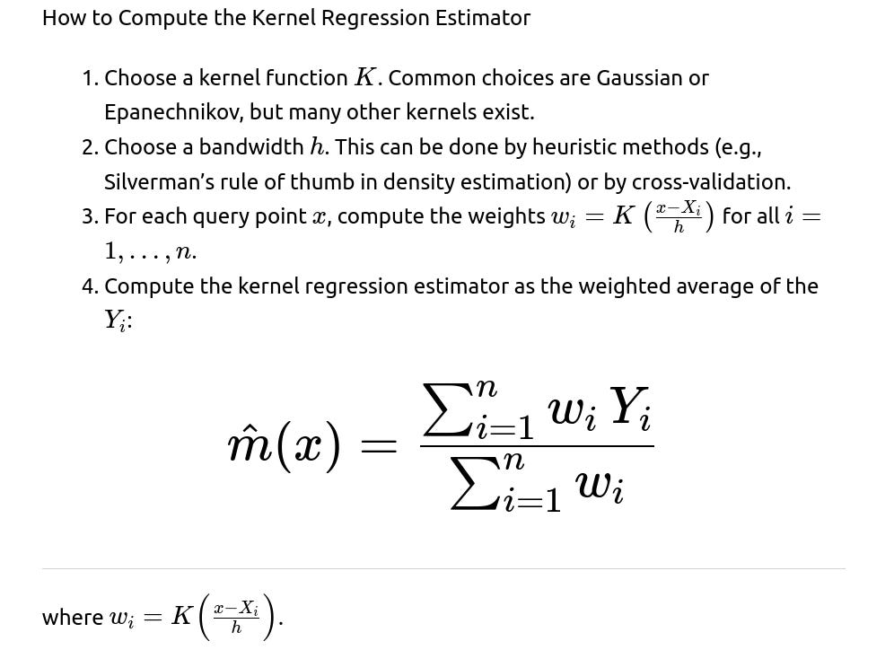
In regression contexts, kernel smoothing often appears as the Nadaraya-Watson kernel regression estimator. This approach replaces the parametric form of regression with a locally weighted average of the observed response values. The underlying principle is:
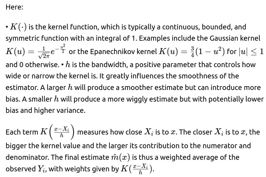
• Each observed data point exerts some influence on the predicted value. • The magnitude of influence depends on a kernel function that decays with distance from the query point. • A bandwidth or smoothing parameter determines how “spread out” the kernel is, controlling the smoothness of the resulting regression curve.
Mathematical Formulation of Kernel Regression
We have a dataset of n observations:

Connection to Local Averaging
Kernel smoothing for regression can be viewed as a localized averaging scheme. To predict at x, you look at data points near x—these get higher weights—while points far from x are down-weighted or practically ignored. This approach is entirely data-driven and does not explicitly assume a global parametric form like linear or polynomial. Instead, we are effectively allowing the shape of the regression function to adjust based on local neighborhoods defined by the kernel.
Example Code in Python
Below is a simple Python snippet to illustrate how you might compute this estimator in practice using, say, a Gaussian kernel. This snippet assumes you have NumPy arrays of features and targets.
import numpy as np

def gaussian_kernel(u):
    return (1/np.sqrt(2*np.pi)) * np.exp(-0.5 * u**2)

def kernel_regression(X, Y, x_query, h):
    # X, Y are arrays of training data
    # x_query is the point at which we want to estimate the regression
    # h is bandwidth
    weights = gaussian_kernel((x_query - X) / h)
    numerator = np.sum(weights * Y)
    denominator = np.sum(weights)
    return numerator / denominator

# Example usage:
X_train = np.array([0.1, 0.4, 0.5, 1.0, 1.2])
Y_train = np.array([2.3, 2.8, 2.5, 3.4, 3.9])
x_query = 0.6
h = 0.2

estimate = kernel_regression(X_train, Y_train, x_query, h)
print("Kernel regression estimate at x=0.6:", estimate)
This simple code demonstrates how you can implement the Nadaraya-Watson estimator with a Gaussian kernel in Python.
Choosing a Kernel Function
The choice of kernel K often matters less than the choice of bandwidth h. Many kernels (Gaussian, Epanechnikov, Triweight, etc.) can yield very similar results in practice as long as they are properly normalized and continuous. Typically, the bandwidth has a much more substantial influence on performance. Nonetheless, in many cases the Gaussian kernel is a default choice due to its smoothness and infinite support.
Practical Considerations in Bandwidth Selection
Choosing the bandwidth h is critical. The typical methods include:
• Cross-validation (e.g., leave-one-out cross-validation): You select an h that minimizes some measure of predictive error. • Plug-in methods: Approximate the “optimal” bandwidth with formulas that involve the data’s distribution. • Ad hoc heuristics or rules of thumb: For example, in density estimation, a widely used rule is Silverman’s rule, though it can also be applied analogously in kernel regression as a starting point.
Because kernel smoothing is a bias-variance trade-off scenario, smaller bandwidth leads to lower bias but often higher variance, while larger bandwidth leads to higher bias but lower variance.
Potential Issues and Pitfalls
• Curse of Dimensionality: Kernel methods can degrade in high-dimensional spaces because neighborhoods become sparse. The kernel might end up with roughly equal weights for many widely spaced points, and the concept of “local” might break down if X has many dimensions. • Boundary Effects: Near the boundaries of the data range, fewer data points lie on one side of the query, which can lead to biased estimates unless boundary corrections are used. • Computation for Large n: Computing the kernel estimator for each query point can be expensive for large datasets, since it typically requires summation across all training points. Approximate methods or specialized data structures (like KD-trees or ball trees) may help scale the computation. • Over-Smoothing vs. Under-Smoothing: If the bandwidth h is too large, the estimator could flatten important structures (over-smoothing). If h is too small, the function could become too wiggly and fit noise (under-smoothing).
Use Cases in Real Applications
• Non-linear trend fitting: Kernel smoothing is especially effective if the relationship is unknown, non-linear, or piecewise. • Density estimation: Closely related kernel smoothing ideas are used in kernel density estimation, which is used in many anomaly detection or data distribution analysis tasks. • Visualization: Kernel smoothing can be used to create a smooth curve in scatter plots for quick insights into the relationship between two variables.
What if the data has multiple features? How does kernel smoothing extend to multiple dimensions?

However, as d grows, the volume of the input space grows exponentially, and you need exponentially more data to maintain a similar density of points. This is often referred to as the curse of dimensionality. Practically, kernel smoothing in high dimensions can become computationally infeasible or statistically inefficient unless you use dimensionality reduction or apply specialized methods that mitigate data sparsity.
How do you handle boundary effects in kernel smoothing?
Boundary effects occur when a query point x lies near the edge of the data domain. In such a case, there are fewer neighbors on one side, so the kernel weights can be skewed and lead to biased estimates. Several strategies address this:
• Reflection: Reflect data across the boundary, effectively pretending there are mirror-image points. • Boundary kernels: Modify the kernel’s shape near boundaries so that its support does not exceed the domain boundary. For instance, in density estimation, the Epanechnikov kernel can be adjusted adaptively at the edges. • Local polynomial regression (e.g., LOESS/LOWESS): Instead of simple averaging with weights, you fit a local polynomial in a small region. This can help reduce boundary bias, as the polynomial can extrapolate properly at the edges.
In practice, if the domain is not sharply bounded or if your data does not lie near a strict boundary, you might not worry too much about boundary effects. But in certain applications (e.g., modeling phenomena that only occur in [0,1]), boundary corrections can be crucial.
How do you use cross-validation to select the bandwidth for kernel regression?
In k-fold cross-validation, you would:

The same principle extends to other loss functions (e.g., absolute error) if that’s relevant to the problem. Cross-validation is computationally more expensive because for each candidate h you’re re-estimating the kernel smoother multiple times, but it is often the most robust method to find a high-quality bandwidth in practice.
Why is the choice of kernel often said to be “less important than the bandwidth”?
Many common kernels (like Gaussian, Epanechnikov, Triweight, etc.) are smooth, continuous, and unimodal, with a single peak at zero. Given these similarities, each kernel tends to produce comparable results when scaled by the same bandwidth, particularly if the data distribution is not pathological. On the other hand, the bandwidth h has a large impact: a small bandwidth leads to a very spiky, potentially overfitted solution, while a large bandwidth can obscure important details, producing an overly smoothed estimate. Thus, the entire shape of the regression function—and the associated bias-variance trade-off—depends strongly on the bandwidth, which is why practitioners often say it matters more than the choice of kernel function.
In real-world ML systems, why might you prefer a parametric or semi-parametric method to kernel smoothing?
Although kernel smoothing is flexible, real-world systems face practical constraints:
• Data size and real-time predictions: Kernel smoothing requires evaluating a sum of kernel functions for each query. For massive n, this can be too slow. A parametric or semi-parametric model can be much faster at inference time once trained. • High dimensions: Kernel smoothing can deteriorate as dimensionality grows, while parametric models might handle high dimensions better if you can guess or engineer a useful functional form. • Interpretability and consistency: Some parametric models come with established interpretability or well-known confidence intervals. Kernel smoothing can be less direct to interpret, especially in multiple dimensions. • Online or streaming data: Kernel methods need to store all (or a large subset of) the training data for predictions. A parametric model typically maintains a fixed number of parameters and is easier to update incrementally.
Semi-parametric or hybrid approaches can combine the advantages of both. For instance, you might use a linear model plus a kernel smoothing term for residuals or adopt local parametric fits like LOESS.
How might you approximate or scale kernel smoothing to large datasets?
For large datasets, naive kernel regression has a runtime complexity of O(n) per query point. If you have a big set of query points, the total complexity can be O(n×(number of queries)). Possible strategies to mitigate this:
• Use tree-based data structures: KD-trees, ball trees, or vantage-point trees can speed up nearest neighbor searches. Once you have an efficient way to find neighbors of x, you can limit the computation to only those data points that have non-negligible kernel weights. • Nyström or random Fourier features: For certain kernels (like Gaussian), you can approximate the kernel function with lower-dimensional feature mappings. You transform your data points into these features and then do approximate kernel smoothing in that transformed space. • Clustering-based approximation: Partition the dataset into clusters, approximate the local distribution within each cluster, and then do a weighted average of cluster-level predictions. • Subsampling: Use a random subset of data to do kernel smoothing, which can still capture local structure if done carefully. • GPU acceleration or parallelism: If memory is not a limiting factor, you can accelerate the summations significantly by parallel processing.
All these methods aim to reduce the computational overhead without sacrificing too much accuracy.
Could you explain the bias-variance trade-off in kernel smoothing?
In kernel smoothing, the bandwidth h embodies the bias-variance trade-off:
• Large h (broad kernel): The estimator averages many points, so random fluctuations due to small sample size or noise are evened out. This lowers variance but can create bias if the true function changes rapidly within the kernel’s width. • Small h (narrow kernel): The estimator focuses on very local neighborhoods. It captures fine details and can reduce bias if the data is dense. However, it can lead to higher variance because the estimator heavily depends on fewer points.
Mathematically, the bias-variance decomposition of the kernel estimator reveals that bias typically increases with h, while variance decreases with h. An optimal bandwidth typically balances these two.
How does kernel smoothing relate to LOESS (or LOWESS) methods?
LOESS (Locally Estimated Scatterplot Smoothing) or LOWESS is a generalization of kernel smoothing where, instead of computing a simple weighted average of Y values, you fit a local polynomial (commonly a linear polynomial) in a small neighborhood around x. This means for each query point x, you solve a weighted least squares problem:

This approach can reduce bias near boundaries and better capture local linear patterns. However, it is computationally more expensive than a simple Nadaraya-Watson average, since a local regression has to be fit around each query point. Despite the extra complexity, LOESS is popular in data exploration for its smoothness and interpretability at small scales.
How is kernel smoothing used in density estimation, and how does that relate to kernel regression?


Why might kernel smoothing be a good fit for a small to medium dataset with a potentially non-linear relationship?
For small to medium-sized datasets with unknown or complicated functional forms, kernel smoothing can be highly flexible and can adapt to local structures without requiring you to guess a global parametric form. When data size is moderate, the O(n) evaluation cost might be acceptable. Also, for lower-dimensional input spaces, the curse of dimensionality is less severe, making kernel smoothing feasible. It often provides an intuitive sense of how the data locally influences the regression estimate, which can be particularly valuable in exploratory data analysis.
When would kernel smoothing break down?
Kernel smoothing might break down if:
• Dimensionality is too high. You have data in, say, 100-dimensional space, and the local neighborhoods might contain too few samples to form reliable estimates. • Data is extremely large, making real-time predictions or repeated queries computationally too expensive. • You face abrupt jumps or discontinuities in the function, and the kernel smoothing’s local averaging might blur these discontinuities unless you shrink h drastically or use specialized discontinuous kernel approaches. • You require interpretability or parametric forms for theoretical reasons, or you need a closed-form solution for inference (e.g., known confidence intervals for parameters).
Below are additional follow-up questions
Are there specialized kernels for time-series data, and how would you apply kernel smoothing in a temporal context?
In time-series analysis, the data has an inherent ordering in time, and often we care about the local temporal neighborhood rather than a purely spatial or feature-based neighborhood. Standard kernels (like Gaussian) can still be used if you treat time t as your input. However, specialized kernels for time-series might incorporate periodicity or domain knowledge about seasonality and trends.
A common scenario is seasonal or cyclic data, such as daily or annual periodic patterns. If you suspect a seasonal component, you might choose a kernel that captures periodic behavior, for example:

In a more advanced approach, you could define composite kernels mixing a standard Gaussian term for local behavior plus a periodic kernel term for seasonal effects.
Pitfalls and edge cases:
If the time series has abrupt changes (e.g., regime shifts), a globally smooth kernel might not capture those transitions well.
Bandwidth selection in a time-series context is tricky because data autocorrelation can produce false confidence that a small bandwidth is sufficient. Cross-validation methods for time-series (like rolling-origin or forward-chaining) are crucial to avoid leakage from future data.
Non-stationary time series might require adaptive bandwidth, where h changes over time to capture evolving structure.
Is kernel smoothing differentiable, and can we use gradient-based optimization with it?

For each x, you need to recompute weights involving all n training points (unless you have an approximate method). This can be computationally expensive.
In high dimensions, you might still suffer from the curse of dimensionality and limited data density in local regions, which can make gradients noisy or uninformative.
Pitfalls and edge cases:
If two (or more) data points are exactly at x and the kernel is extremely peaked, you could have numerical issues in the denominator.
For bandwidth approaches that set h adaptively per x (e.g., nearest neighbor bandwidth selection), the derivative can get complicated.
How do you measure uncertainty or construct confidence intervals in kernel smoothing?
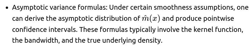
Because kernel smoothing is nonparametric, classical parametric formulas for confidence intervals do not directly apply. Several methods exist:
Bootstrap methods: Resample the dataset (e.g., by drawing n points with replacement), recompute the kernel smoother for each bootstrap sample, and measure the variability in the resulting estimates at each x. This is straightforward conceptually but can be computationally expensive.
Jackknife or leave-one-out approaches: Similar in spirit to bootstrap, but specifically removing each observation once to measure variability.


Pitfalls and edge cases:
For small n, the asymptotic approximations might not be accurate, so you should rely more on bootstrap methods.
Heteroskedastic data (i.e., the variance of Y changes with X) requires more careful handling. Standard kernel smoothing might not account for it directly, so standard confidence interval formulas may be inaccurate.
How robust is kernel smoothing to outliers or heavy-tailed distributions?

Can you perform variable selection or feature importance estimation within kernel smoothing for high-dimensional inputs?
Traditional kernel smoothing is not inherently designed to do variable selection because it treats all features equivalently within the distance measure. However, several extensions exist:

Hybrid or two-stage methods: For instance, you could run a random forest or gradient boosted trees to identify important features, then apply kernel smoothing using only the top d features or reweigh them accordingly.


Pitfalls and edge cases:
Estimating a full matrix bandwidth H is challenging; naive methods scale poorly for large d.
Regularization or feature selection steps might reduce interpretability of the final kernel smoother because you have two (or more) sets of hyperparameters: the bandwidth and the penalty terms.
What if the underlying function is known or expected to be monotonic? Does kernel smoothing guarantee monotonicity?
Kernel smoothing with a standard kernel does not guarantee any specific shape (like monotonic increase/decrease). It is fundamentally a local averaging procedure, so if the data points around x happen to produce a non-monotonic pattern, the kernel estimate will reflect that.
If you need a monotonic function:
You might impose constraints in a local polynomial fit (constrained local regression) ensuring the slope remains nonnegative (or nonpositive).
Post-processing step: After fitting a kernel smoother, you can enforce monotonicity by projecting the estimated function onto the set of monotonic functions. This can be done via an isotonic regression approach on the predicted values.
Pitfalls and edge cases:
Imposing monotonic constraints could introduce boundary artifacts or kinks where the function is forced to maintain or revert to monotonic behavior.
If the data truly has non-monotonic sub-regions, forcing monotonicity can introduce large bias in those regions.
Can we adapt kernel smoothing for classification tasks, such as binary or multi-class classification?
Yes, you can extend kernel smoothing to classification by using local voting or local likelihood. In binary classification, a straightforward approach is:

Pitfalls and edge cases:
If data is highly imbalanced, local averaging might produce overly smoothed probabilities near minority class regions.
If the classes are not well-separated in feature space, a very small bandwidth might be needed to preserve local distinctions, but that can lead to high variance in the estimated probabilities.
Are there practical libraries or built-in functions in Python for kernel smoothing, and what are some implementation details?
statsmodels: Offers nonparametric kernel regression in
statsmodels.nonparametric.kernel_regression. You specify the bandwidth, kernel type, etc.scikit-learn: Has kernel density estimation functionality in
KernelDensity, but not a direct built-in for kernel regression. You’d typically roll your own or use other libraries or code snippets.PyTorch / TensorFlow: You can implement kernel smoothing using vectorized operations on the GPU if you want. This is particularly beneficial for large datasets or repeated queries. However, you typically have to code your own routines or rely on specialized custom packages.
Implementation details:
Vectorizing computations is crucial for speed. Instead of looping over points, you can compute distances in a matrix form (broadcasting in NumPy/PyTorch).
Caching repeated computations (e.g., the kernel matrix if you query multiple x points) can save runtime but may be memory-intensive for large n.
For multivariate data, consider how you handle the distance metric—L2 distance is common, but other metrics might be more appropriate for certain data types.
Pitfalls and edge cases:
Memory constraints if you form a large n×n kernel matrix.
Numerical stability issues if h is extremely small or extremely large.
GPU usage must be carefully managed if the dataset does not fit in GPU memory at once.
How can kernel smoothing be leveraged for residual analysis or partial dependence in advanced ML pipelines?
Sometimes kernel smoothing is used as a post-processing or exploratory technique:

How can kernel smoothing be adapted to streaming data with concept drift?
Concept drift occurs when the data distribution changes over time. For kernel smoothing in a streaming setting:
One approach is to use a moving window of recent data, discarding older data points. The kernel regression is then performed only on the most recent W points. This ensures your estimate stays current if the concept changes.
Another approach is to down-weight older points by a decay factor. This can be viewed as an exponential smoothing approach within a kernel framework.
Adaptive bandwidth selection might also help if the variability changes over time. You can tune h on a rolling basis using a short-window cross-validation.
Pitfalls and edge cases:
If concept drift is abrupt (e.g., sudden switch in the generative process), even a kernel smoother with a short memory might not immediately capture the new regime unless you have a mechanism to detect and reset the model.
If the concept drift is slow, a too-aggressive forgetting mechanism might throw away relevant older data.
Are kernel smoothing techniques related to radial basis function networks in neural networks?
Radial Basis Function (RBF) networks are indeed related to kernel smoothing. In an RBF network:
Hidden units are radial basis functions, often Gaussian-shaped, centered at certain “prototype” points.


The output layer is typically a linear combination of these hidden units.
In kernel regression, each data point effectively acts like a “center” with a Gaussian (or other kernel) shape. The difference is that kernel smoothing typically uses all data points as centers, whereas an RBF network might learn a smaller set of centers or use clustering to reduce complexity.
Pitfalls and edge cases:
An RBF network can become computationally expensive or overfit if you use one radial basis unit per data point (like in kernel smoothing).
There is a separate training process in an RBF network to learn center locations and possibly widths. In kernel smoothing, the “centers” are just the training points, and the bandwidth is a hyperparameter you tune.
How do you incorporate heterogeneous data point reliability or weighting in kernel smoothing?

This way, points with higher reliability or importance weigh more in the local average.
Pitfalls and edge cases:

How might kernel smoothing handle discrete or categorical features?
Kernel smoothing is most straightforward for continuous numeric features where distance-based kernels make intuitive sense. For discrete or categorical features:
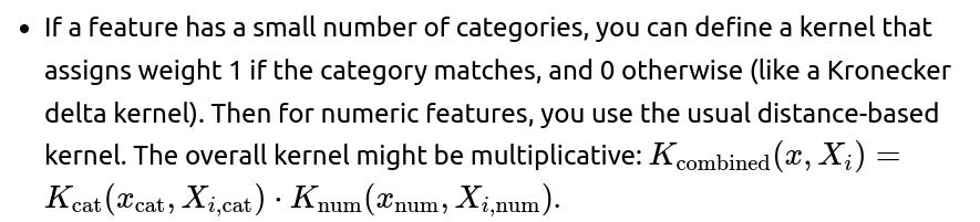
For higher-cardinality categorical features, or if the categories have some known distance metric (like geographical regions), you could define an appropriate similarity measure and embed that into a kernel.
Pitfalls and edge cases:
If categories are purely nominal with no natural ordering, you have to define distance or similarity heuristics carefully.
If there are many categories with sparse data, the local neighborhoods might become too small to be meaningful. This is similar to the dimensionality issue but with discrete dimensions.
Could kernel smoothing be used for anomaly or novelty detection?
Yes, you can adapt kernel smoothing for anomaly detection by doing something akin to kernel density estimation:

Pitfalls and edge cases:
You need enough samples in all relevant regions to have a meaningful density or regression reference.
In high dimensions, density estimates can be extremely low or unreliable because of data sparsity.
Are there any ways to accelerate queries if you need to perform repeated kernel smoothing predictions on many query points?
Precompute and store distances: If the query points are fixed or known in advance, you could store all pairwise distances or partial sums. However, this is ParseError: KaTeX parse error: Expected 'EOF', got '#' at position 18: …n \times \text{#̲queries}) in space, which might be impractical for large n.

Approximate nearest neighbor methods: Tools like hierarchical navigable small world graphs (HNSW) or LSH-based approaches let you rapidly find neighbors in higher dimensions with approximate search.
Grid-based approximation: If the input domain is low-dimensional (like 1D or 2D), you can discretize and precompute kernel sums on a grid, then interpolate the result. This is popular for smooth function approximation tasks.
Pitfalls and edge cases:
Tree-based methods degrade in very high dimensions as all points become distant neighbors.
Approximate methods can introduce errors in the kernel sums, but might be acceptable if you only need approximate predictions.
Grid-based approaches become infeasible if dimension is greater than 2 or 3, due to exponential growth in grid points.