ML Interview Q Series: Normal Approximation of Binomial Probabilities via the Central Limit Theorem

Browse all the Probability Interview Questions here.

Question

N independent trials are to be conducted, each with success probability p. Let Xᵢ = 1 if trial i is a success and Xᵢ = 0 if it is not. What is the distribution of the random variable X = X₁ + X₂ + ... + X_N? Express P(a ≤ X ≤ b) as a sum (where a < b and these are integers between 0 and N). Use the central limit theorem to provide an approximation to this probability. Compare your approximation with the limit theorem of De Moivre and Laplace on p.1189 of Kreyszig.

Short Compact solution

X is the total number of successes in N independent trials, so X follows a Binomial(N, p) distribution. Therefore:

Because each Xᵢ has expected value p and variance p(1 − p), the Central Limit Theorem (CLT) implies that for large N, X can be approximated by a Normal(Np, Np(1 − p)). Defining

ā = (a − Np) / √[N p(1 − p)]

and

b̄ = (b − Np) / √[N p(1 − p)],

we approximate

P(a ≤ X ≤ b) ≈ P(ā ≤ Z ≤ b̄),

where Z is a standard Normal(0, 1) random variable. A continuity correction can improve the accuracy, often implemented by replacing a and b with a − 0.5 and b + 0.5, respectively. This is consistent with the presentation in Kreyszig, where a “small correction” δ in (0, 1) is introduced.

Comprehensive Explanation

Understanding the Binomial Distribution X represents the count of successes in N independent Bernoulli trials, each with probability p of success. A Bernoulli trial is simply a random event that takes the value 1 with probability p or 0 with probability 1 − p. Summing these N independent Bernoulli outcomes, we obtain X, which has the Binomial distribution Binomial(N, p).

The PMF (Probability Mass Function) of a Binomial(N, p) is given by the binomial coefficient multiplied by the appropriate powers of p and 1 − p. Specifically, for integer x from 0 to N, the probability that X = x is (N choose x) p^x (1 − p)^(N − x).

Hence, to compute P(a ≤ X ≤ b) exactly, one sums the binomial probabilities from x = a to x = b:

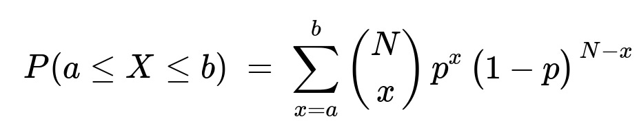
where 0 ≤ a < b ≤ N.

Key Parameters of the Binomial Distribution Because X is the sum of N independent Bernoulli(p) random variables, its expected value is Np and its variance is Np(1 − p).

Approximation via the Central Limit Theorem When N is large, even though the underlying distribution is discrete, the Central Limit Theorem tells us that X can be well approximated by a continuous normal distribution with mean Np and variance Np(1 − p). In other words, X ≈ Normal(Np, Np(1 − p)).

To find P(a ≤ X ≤ b) using this Normal approximation, we standardize X by subtracting its mean and dividing by its standard deviation √[N p(1 − p)]. Concretely, define

ā = (a − Np) / √[N p(1 − p)] b̄ = (b − Np) / √[N p(1 − p)],

and note that (X − Np)/√[N p(1 − p)] behaves approximately like a standard normal variable Z with mean 0 and variance 1. Thus,

where Φ denotes the cumulative distribution function (CDF) of the standard Normal(0,1).

Continuity Correction (the “Small Correction”) Because the Binomial distribution is discrete and the Normal distribution is continuous, more accuracy can often be gained by applying a continuity correction. One common approach is to replace a and b in the above probability with a − 0.5 and b + 0.5, respectively, to account for the fact that X jumps in discrete units.

Hence, a refined approximation is:

P(a ≤ X ≤ b) ≈ Φ((b + 0.5 − Np)/√[N p(1 − p)]) − Φ((a − 0.5 − Np)/√[N p(1 − p)]).

This is the correction mentioned in Kreyszig, where you introduce a small δ in (0,1). Typically, δ = 0.5 is used.

Comparison to the De Moivre–Laplace Theorem The De Moivre–Laplace theorem is essentially the binomial form of the CLT for p = 1/2 or a more general p, and states that as N becomes large, the binomial distribution Binomial(N, p) converges to the appropriate Normal distribution with the same mean and variance. This is precisely the underpinnings of our approximation above.

Follow-Up Question: When is the Normal Approximation to the Binomial Distribution Inaccurate?

For the Normal approximation to be reliable, N should be “sufficiently large,” and p should not be too close to 0 or 1. A common heuristic is to require Np ≥ 5 and N(1 − p) ≥ 5 as a rough rule of thumb. When p is extremely small or extremely large (p near 0 or 1), the binomial distribution can become highly skewed, making the symmetric normal approximation less accurate unless N is very large.

In cases where p is very small and N is also large in such a way that the product λ = Np remains moderate, you might use a Poisson approximation instead.

Follow-Up Question: What is the Role of Continuity Correction in More Detail?

A continuity correction helps bridge the gap between a discrete distribution (Binomial) and a continuous one (Normal). For instance, if you want P(X ≤ k) for a binomial variable X, the uncorrected normal approximation uses P(Z ≤ (k − Np)/√[N p(1 − p)]). But X ≤ k means X can take any integer up to and including k. In continuous space, that entire binomial “mass” from X = k to X = k+1 should be captured in the approximation. By introducing a shift of +0.5 to k, you approximate the half-integer boundary around k, improving the match between discrete sums of probabilities and the integral under a continuous curve.

Follow-Up Question: Can We Derive the Error Bounds for the Normal Approximation?

There are known bounds on the error of the normal approximation, often coming from Berry–Esseen–type theorems, which measure how quickly the distribution of a standardized sum converges to the normal distribution. The simpler form of these bounds typically depends on higher-order moments of the underlying Bernoulli variable and can show that the convergence error decreases on the order of 1/√N.

In practice, most texts rely on empirically tested rules of thumb (such as Np ≥ 5, N(1 − p) ≥ 5, or using continuity corrections) rather than presenting exact error bounds. For FANG-level interviews, it is often enough to demonstrate understanding that there are formal bounds involving the third central moment or cumulants, and that these bounds shrink with increasing N.

Follow-Up Question: How Would We Implement This Approximation in Python?

In Python, we can compute the exact binomial probabilities using libraries like scipy.stats. For larger N, it can become costly or prone to underflow/overflow in direct computation of (N choose x) p^x (1 − p)^(N−x). In that case, we can switch to either the normal approximation or use specialized functions for the binomial CDF.

Below is a simple example illustrating how to compare the exact Binomial CDF with the Normal approximation:

import numpy as np
from math import sqrt, exp, pi
from scipy.stats import binom, norm

N = 100
p = 0.3
a, b = 20, 40

# Exact Binomial probability
exact_prob = binom.cdf(b, N, p) - binom.cdf(a - 1, N, p)

# Normal Approximation
mean = N * p
var = N * p * (1 - p)
std = sqrt(var)

# With continuity correction
a_cc = a - 0.5
b_cc = b + 0.5

approx_prob = norm.cdf((b_cc - mean)/std) - norm.cdf((a_cc - mean)/std)

print("Exact Binomial Probability:", exact_prob)
print("Normal Approx (continuity-corrected):", approx_prob)

In a real interview, demonstrating awareness of numerical stability (for instance, using binom.logpmf for large N) and the ability to choose between exact and approximate distributions based on problem constraints will highlight a strong understanding of practical details in probabilistic modeling.