
ML Interview Q Series: Normal Distribution Threshold Wait Time: A Geometric Distribution Analysis

Browse all the Probability Interview Questions here.
You draw a single sample each day from a normal distribution with mean 0 and standard deviation 1. Approximately how many days do you expect to pass before observing a value that exceeds 2?
Short Compact solution
We use the fact that a standard normal random variable has the cumulative distribution function (CDF) value at 2 of about 0.9772. Consequently, the probability of drawing a value greater than 2 on any given day is 1 − 0.9772 = 0.0228. Because each draw per day is independent, the waiting time follows a geometric distribution with success probability 0.0228. The mean waiting time for a geometrically distributed random variable with parameter p is 1/p. Hence, on average, you would wait about 1 / 0.0228 ≈ 43.86 days.
Comprehensive Explanation
Why the Probability is Computed as 1 − Φ(2)
A normally distributed random variable with mean 0 and standard deviation 1 is called a standard normal. Its distribution is commonly denoted as X ~ N(0,1). The CDF of a standard normal variable at a value x is often written as Φ(x). This CDF gives the probability that X is less than or equal to x. Therefore, the probability of obtaining a value greater than 2 is:
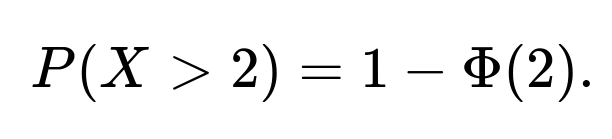
Using standard normal tables, software (e.g., Python’s scipy.stats), or well-known approximations, we find that Φ(2) ≈ 0.9772, implying P(X > 2) ≈ 0.0228.
Why the Waiting Time Follows a Geometric Distribution
When you perform the same independent experiment repeatedly each day, waiting for the first success (where “success” = drawing a value > 2), the number of trials until the first success follows a geometric distribution. Key points include:
Independence: Each daily draw from N(0,1) does not affect the next day’s draw.
Same success probability: The probability of success (value > 2) remains constant at 0.0228 every day.
This setup precisely matches the definition of a geometric random variable.
Expected Value of the Geometric Distribution
If a random variable T follows a geometric distribution with success probability p (in our case p = 0.0228), the expected value is given by:

Here, we substitute p = 0.0228, giving:
E[T] = 1 / 0.0228 ≈ 43.86.
Hence, on average, it will take around 44 days to observe the first sample exceeding 2.
Connection to Real-World Interpretations
Interpreting this result, if you are performing one draw per day from a standard normal distribution, you should expect to wait slightly over six weeks on average before you get a value bigger than 2. Of course, “on average” means that in some runs you might see a value over 2 in just a few days, and in others it might take considerably longer. But over many repeated trials, the mean waiting time converges to about 43–44 days.
Potential Follow-Up Questions
Why does the waiting time have the memoryless property?
The geometric distribution is known for its memoryless property, meaning that if you have been drawing for many days without success, the probability of success on the next draw is still p (0.0228 in our case), unaffected by how long you have already waited. This arises from the independence of daily draws and the unchanging probability p each day.
What if the daily draws were not independent?
If the draws were correlated, the waiting-time distribution might no longer be geometric. For example, if a higher-than-average outcome today makes it more likely that tomorrow’s draw is also above average, that correlation would affect the probability of hitting a value over 2. The exact distribution in such a correlated scenario would need deeper modeling, and the simple formula 1/p for the mean waiting time would not directly apply.
How do we verify the normality assumption in practice?
In real scenarios, we often check whether samples come from a normal distribution using techniques like Q-Q plots, the Kolmogorov–Smirnov test, or the Shapiro–Wilk test. If data diverges substantially from normality, we would re-estimate or reevaluate the probability of exceeding 2 using the actual distribution.
How can we calculate or approximate Φ(2) if we do not have tables or software?
We can use numerical approximations such as expansions of the error function (erf) or rational approximations found in many textbooks. One common approximation for Φ(x) is based on a polynomial or rational function fit, but in a coding context, a standard library (e.g., scipy.stats.norm.cdf in Python) is typically used for convenience and accuracy.
Could we estimate this probability from data if the distribution were unknown?
If we lack the assumption of normality, one approach is to gather empirical data from repeated draws (or from a real-world process). We could then estimate P(X > 2) by counting how frequently values exceed 2. This empirical probability can be plugged into a geometric distribution framework if independence and identical distribution hold. The reliability of the estimate depends on having enough data to capture tail behavior accurately.
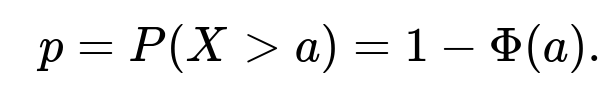
What if the threshold changes or we need a different quantile?
The same reasoning can be generalized: if you have a threshold a, you compute P(X > a) = 1 − Φ(a) for a standard normal or the corresponding distribution function if the variable is not standard normal. Then 1/p yields the expected waiting time for that threshold. If a were larger (e.g., 3), you would get a smaller p and a larger expected waiting time.
How can we simulate this scenario in code to confirm?
A quick Python simulation approach is:
import numpy as np

np.random.seed(42)
num_simulations = 10_000_00  # number of trials
threshold = 2

days_to_exceed = []

for _ in range(num_simulations):
    count_days = 0
    while True:
        count_days += 1
        x = np.random.randn()  # draw from N(0,1)
        if x > threshold:
            days_to_exceed.append(count_days)
            break

print("Average days to exceed 2:", np.mean(days_to_exceed))
This simulation would converge to a value near 44 days as the number of simulations grows.
Below are additional follow-up questions
What if the threshold we are looking for is below the mean (e.g., a value less than 0)? Would our approach change?
When the threshold is below the mean, say a < 0, the probability of exceeding that threshold is much higher than when a = 2. In such a scenario, let’s denote the threshold by a. We compute:
Because a < 0, the value of Φ(a) is less than 0.5, and thus 1 − Φ(a) is more than 0.5. This probability p could be quite large (e.g., if a = −1, the probability might be well over 0.84). If p is large, the expected number of days until exceeding a is much smaller. In practice, the same geometric distribution approach remains valid:
Each day’s draw is independent, and the probability of success is p = 1 − Φ(a).
The expected waiting time is still 1/p.
The only real difference is that because p is relatively large, you’d expect to see a value larger than a after only a few days on average. The approach does not change; the outcome changes simply because the probability is now higher.
A potential pitfall arises if you get confused about whether you’re dealing with “exceeding a lower threshold” or “falling below that threshold.” Here, we strictly need P(X > a). If we wanted P(X < a) instead, we would use Φ(a). This is mainly a matter of carefully defining your event of interest.
How would sampling multiple times per day (instead of once a day) affect the analysis?
If you take multiple independent draws each day, you can think of the number of “mini-trials” within one day as multiple Bernoulli experiments (with the same probability p = P(X > 2) for each draw). If you define “success” as seeing at least one value above 2 in a single day, and you perform m independent draws per day, then the probability of success in a single day becomes:
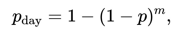
where p is the probability that a single draw exceeds 2. In that case, the waiting time (in days) until you get your first daily success (i.e., at least one draw above 2 on that day) is still geometrically distributed, but with parameter ( p_\text{day} ) instead of p. The expected number of days to see a success day is then:

A subtle pitfall is that you need to distinguish between “the first time we see a value above 2 in any draw” (which might be mid-day) and “the first day in which we see a value above 2 in at least one of that day’s draws.” If you care about the exact moment, you might treat each draw as a separate trial with a geometric distribution that no longer maps directly to a “day count” but rather to a “draw count.” To convert to days, you would note the average number of draws until success and then see how that translates into days (e.g., if you have 10 draws per day, the expected number of draws until success is 1/p, and then you could divide by 10 to interpret it in days).
Could the geometric model break down if the distribution changes over time (non-stationarity)?
Yes. The key assumption in using a geometric model for waiting time is that each trial (day) has the same probability of “success.” If the distribution parameters (mean, variance) shift over time, the probability of exceeding 2 may vary day to day. This scenario is referred to as non-stationary or time-dependent.
In real-world contexts—especially in finance, weather modeling, or any system subject to drift or seasonality—the distribution might change. If, for example, the mean drifts upwards over time, then the chance of exceeding 2 may increase each day. As a result, the probability of success is not constant. The memoryless property of the geometric distribution does not hold, and one might need to model the process with more sophisticated time-series methods or a varying-parameter approach.
Are there scenarios where the geometric distribution might be confused with other discrete distributions?
Yes. Another commonly encountered discrete distribution is the negative binomial distribution, which models the number of trials needed to achieve r successes. Geometric distribution is essentially the special case of the negative binomial for r = 1. If someone accidentally used a negative binomial distribution when only a single success event (the first time exceeding 2) is relevant, they could get incorrect estimates of the waiting time.
Additionally, one might confuse a geometric distribution with a Poisson process for continuous-time events if the question was framed incorrectly. Poisson processes typically apply to counts of events in continuous time, while geometric distributions apply to counts of discrete trials. Mixing these up can happen if you forget that we are only sampling once per day (or in discrete intervals) rather than in continuous time.
What if we want to compute not just the mean waiting time but other metrics like variance or a confidence interval for T?
For a geometric random variable T with parameter p, the variance is given by:

In our scenario with p = 0.0228, the variance is:
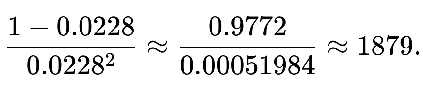
The standard deviation is then the square root of 1879, which is around 43.33. So even though the mean is about 44 days, the standard deviation is of similar magnitude, implying a high amount of variation. Realizations can vary quite widely around the mean, from very few days to hundreds of days.
A confidence interval for the mean waiting time can be derived via standard methods for means of positive random variables or bootstrapping if you have simulated data. An important subtlety here is that the theoretical mean is 1/p. But a single “realization” of T is not an average in the typical sense; it is just the waiting time for that one run. If you run many experiments or do a Monte Carlo simulation, you can build up a distribution of average waiting times and construct confidence intervals from that.
How would truncation or censoring of data affect these calculations?
In some real-world cases, you might only observe a process for a limited time frame (censoring). For instance, you might only be able to record 30 days, and if you haven’t yet drawn a value above 2, you stop. This scenario means you don’t observe the full waiting time in all cases. Traditional geometric calculations assume you can wait indefinitely. With truncated or censored data, the maximum-likelihood estimation of p can be biased if you ignore that truncation. You would have to employ special statistical techniques (e.g., survival analysis for discrete-time data) to account for individuals (or trials) that did not experience the event before the study ended.
Could outlier handling or measurement errors affect the probability of exceeding 2?
In practice, if the measurement system occasionally produces faulty readings (e.g., sensor spikes or software glitches), those might artificially inflate the frequency of “values above 2.” If a fraction of these events are spurious, the estimate of p might be overly large. One might need to filter out anomalies or verify them before concluding that the event “X > 2” truly occurred. This is particularly important when the real data or measurement pipeline is noisy or susceptible to errors. Proper data-cleaning protocols and anomaly-detection mechanisms are therefore essential to avoid misestimating the waiting time.
How might we extend the analysis to a bivariate or multivariate setting?
Suppose we don’t draw a single number each day but a vector of values (e.g., temperature and humidity). We might then define success as the event that a certain function of that vector (e.g., a linear combination or some norm) exceeds a threshold. If the vector is multivariate normally distributed, we need to compute:

where R is a region in the vector space (for instance, the set of points whose norm exceeds 2, or a linear combination that exceeds 2). The exact geometry of R and the covariance matrix of the multivariate normal will influence p. Once p is computed, if each day’s vector draw is independent of previous days, the waiting time is still geometric, and the expected time is 1/p. However, calculating p might be less trivial, requiring numerical or simulation-based methods. A key pitfall is incorrectly applying formulas that only work for the univariate case.
If we only track “the maximum value so far,” can we still use the geometric model?
Tracking the maximum value up to day n is a slightly different view: You’re looking at the sequence of daily maxima, and you stop when the daily maximum first exceeds 2. Although the definition changes from “on day i, do I see a value > 2?” to “by day i, have I seen a value > 2?”, in discrete-time settings with one draw per day, these are effectively the same statement. But if you consider continuous-time tracking of maxima with multiple observations per day, you need to be careful about how you define the event “the maximum so far has exceeded 2.” If each day is truly a single sample, we haven’t changed the scenario. But if you have multiple samples per day and you track the maximum, the probability that the maximum of multiple samples each day is > 2 changes, which leads to the scenario where p is replaced by 1 − (1 − p)^m as discussed above.
When you roll everything up into “the maximum value up to a certain point,” it might be simpler in some contexts just to view each day (with all its draws) as a single Bernoulli trial. The subtlety is in ensuring you’re not double-counting or ignoring times within the day if you’re sampling more frequently than once a day.
What if we don’t have a normal distribution but some heavy-tailed distribution?
Heavy-tailed distributions, such as Pareto or distributions with an α-stable law, can have much greater probability mass far out in the tails compared to the normal distribution. The probability of exceeding 2 might be significantly higher or lower depending on the tail shape. Moreover, some heavy-tailed distributions might not even have finite variance or other standard moments. In such cases:
You would compute p = P(X > 2) using the appropriate CDF.
The waiting time could still be geometric if each draw remains independent with the same p.
However, the normal assumption would no longer hold, so you’d need a different formula for P(X > 2).
A common pitfall is to assume normality without verifying that the data genuinely resemble a normal distribution. Especially in financial returns or certain network traffic data, heavy-tailed behavior is more common, which can significantly change the waiting time distribution.