ML Interview Q Series: Objective Function Derivation for Linear Regression Under Gaussian Input Noise
📚 Browse the full ML Interview series here.
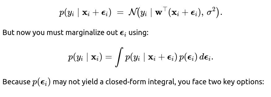
Say we are running a probabilistic linear regression which does a good job modeling the underlying relationship between some y and x. Now assume all inputs have some noise ε added, which is independent of the training data. What is the new objective function? How do you compute it?

Below is an in-depth explanation of why and how this happens, as well as a step-by-step derivation of the new objective function. After that, we explore several related follow-up questions that might come up in a rigorous interview setting.
The usual setup in probabilistic linear regression When we say "probabilistic linear regression," we typically assume that:
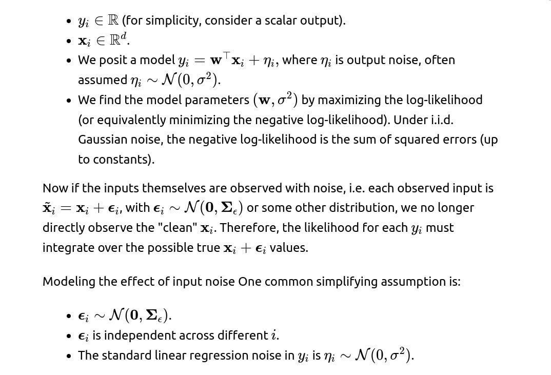
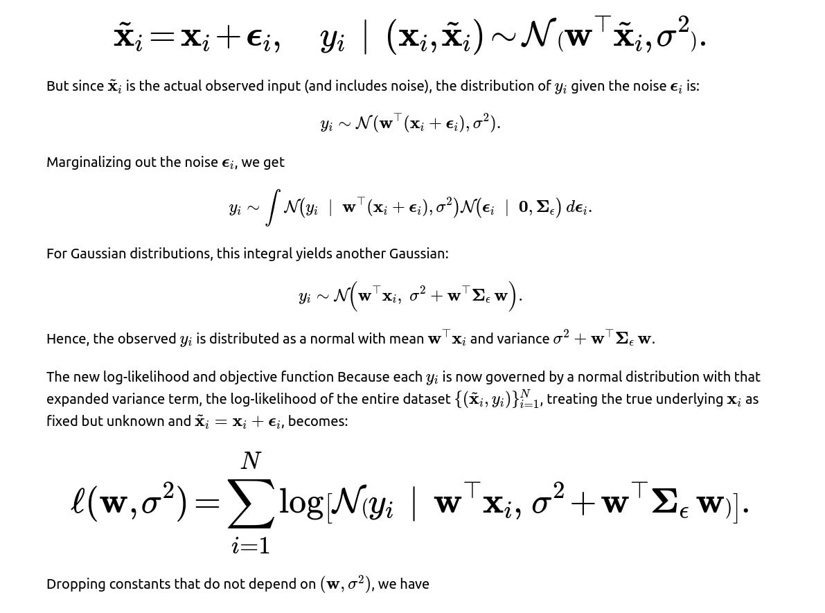
Then our generative process can be described as:


How to interpret the new variance term

Typical pitfalls and real-world considerations

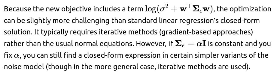
Additional subtle points about the objective
Potential Interview Follow-Ups
Below are several follow-up questions an interviewer might ask, and detailed explanations on how to answer them.
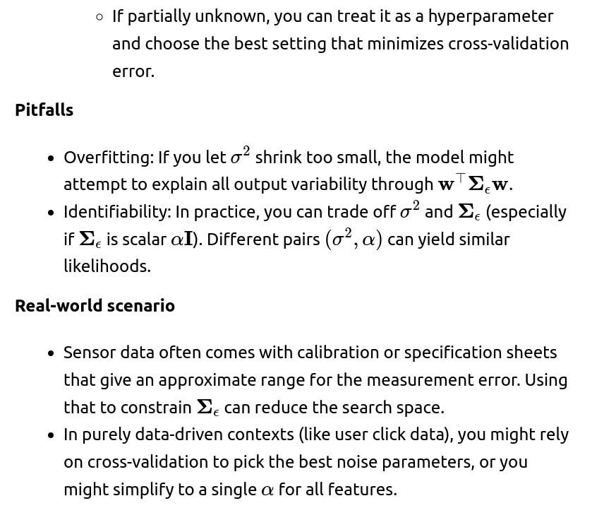
If I do not know the distribution of the input noise, can I still estimate the new objective?

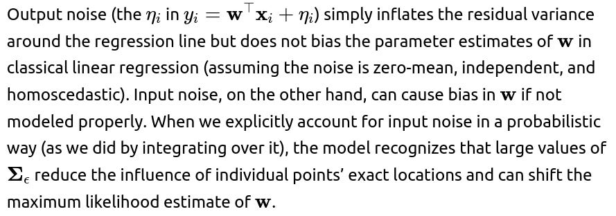
How does input noise differ from output noise in terms of the effect on the estimates of w?


Could we simply do a data augmentation trick where we draw many realizations of the noisy inputs and average the likelihood?
Yes, conceptually one can approximate:

Edge Cases that might trip you up

Additional follow-up questions
If the noise in the inputs is not Gaussian, how would you derive or approximate the objective function?
When we assume Gaussian input noise, we obtain a neat, closed-form expression for the marginal distribution over the observed outputs. However, real-world data may not adhere to Gaussian assumptions. For instance, sensor noise might be better modeled by a heavy-tailed distribution (e.g., Student’s t), or images might have noise that is more complex (e.g., salt-and-pepper noise, which is discrete in nature).
To handle a non-Gaussian input noise distribution, denote it by some density function p(ϵ) that does not necessarily belong to the Gaussian family. The conditional distribution of the output, given the true (but unobserved) x, is still:
Numerical Integration or Quadrature
In low dimensions of x, you might attempt a numerical approximation (e.g., Gauss-Hermite quadrature or Monte Carlo integration).
This approach can be computationally expensive when the dimension of x is large.
Approximate Inference

Potential pitfalls
If the true noise distribution is extremely heavy-tailed (like Cauchy), extreme outliers in xx-space can dominate the objective. A naive model might yield poor or unstable estimates for ww.
If your integration or sampling approach is not thorough, you might fail to capture the tails or multimodal aspects of

Real-world subtleties
In many applied problems (e.g., sensor or signals data), approximate Gaussian noise is a decent assumption. But if you suspect strongly non-Gaussian characteristics (e.g., random occlusions in images), a specialized noise model or robust approach can be crucial.
The dimension of x is a big factor: a high-dimensional input with a complicated noise distribution is much harder to integrate out than a low-dimensional one.
How would you incorporate regularization into this new noise-aware objective?
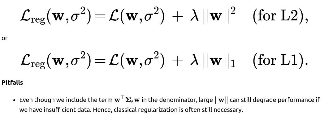
When input noise is included in the model, we might still want to prevent overfitting or control the complexity of the solution. For instance, L2 regularization (Ridge) or L1 regularization (Lasso) is often used in linear regression. In the noise-aware scenario, you have a negative log-likelihood of the form:

You can augment this with a regularization term on w:

Overly strong regularization might cause underfitting, especially if your input noise variance is also large, leading the model to be too conservative.


Real-world considerations

In high-dimensional or extremely sparse domains (like text features), L1 regularization can help enforce sparsity, but with input noise, be aware that some “weak” features might appear noisy but are actually relevant.
What if the input noise is correlated across features (off-diagonal terms in Σε) or correlated across samples?


Pitfalls
Incorrectly assuming independence of input noise across features or samples can bias your parameter estimates and produce overconfident predictions.
Estimating a large covariance matrix Σϵ from limited data is challenging and can lead to overfitting if not regularized.
Real-world examples
Sensor arrays or multi-camera setups can have correlated measurement errors.
Time-series data often have temporal correlations in input noise (e.g., drift).
Genomic data might have correlated measurement errors across genes or loci.
How would you extend this to non-linear models like neural networks or kernel regression?

For Gaussian p(ϵ), this integral might still be intractable for an arbitrary f. One approach is to approximate f(x+ϵ) using a first-order Taylor expansion around xx. Another is to use sampling:
Sampling-based approach: For each training sample, draw several ϵ realizations, evaluate f(x+ϵ;θ), and average the likelihood.
Stochastic gradient variational inference: Treat x itself as a latent variable with some prior distribution. Then approximate the integral with a reparameterization trick if feasible.
Pitfalls
Non-linearities can interact strongly with input noise, making the resulting distribution of y highly non-Gaussian or multi-modal.
Large-scale neural networks might require high computational overhead if you do repeated sampling for each data point.
Real-world subtleties
Certain domains (like computer vision) often rely on data augmentation to simulate noisy or perturbed inputs. That’s effectively a sampling approximation to handle input variability.
Bayesian neural networks might incorporate this concept implicitly if you place a prior on the inputs or treat them as random variables in the model.
If part of the input is known precisely and only some features are noisy, how does that change the modeling?
Often in practice, only certain sensors or fields in your data pipeline are unreliable. For instance, you might have:


Pitfalls
Ignoring which features are truly noisy can lead to suboptimal results. If only half of your features have noise, modeling them all as noisy inflates the variance unnecessarily.
Overlooking small but non-negligible noise in the “clean” part can introduce bias if that portion is not truly noise-free.
Real-world examples
In medical data, some measurements (like patient age) might be exact, while others (like certain lab results) have measurement errors.
In environmental sensor arrays, temperature might be precise while humidity is known to have more drift or random noise.
How does the new noise-aware objective interact with outlier detection or robust regression methods?
In classical linear regression, robust methods (like Huber loss or Student’s t-based regression) are introduced to handle outliers in y. But if you have outliers or anomalies in x (i.e., certain observations are far from typical x even after accounting for noise), or if the noise distribution has heavy tails, you might adopt robust distributions for the input noise itself.
Robust in x-space: Suppose you use a heavy-tailed prior for ϵ (like a Student’s t). That can reduce the influence of extreme input deviations.
Combined robust approach: You can also simultaneously make the output noise or the likelihood function robust if you suspect outliers in y.
Pitfalls
A mismatch between the chosen robust distribution and the actual data distribution can degrade performance.
Tuning robust parameters (like degrees of freedom in a Student’s t) can be non-trivial and data-dependent.
Subtle real-world scenario
In sensor networks, certain times or certain devices might produce sporadic spikes in both x and y. Handling this scenario might require robust methods for both input and output simultaneously, plus a way to detect systematically malfunctioning sensors.
How could you handle partial labeling where some y values are missing but inputs (noisy or otherwise) are still observed?

If the labeled data is not representative (e.g., missingness is not random), that can bias your parameter estimates.
Real-world complexities
In large-scale industrial settings, you might have data streams of features but only sporadic labeling events.

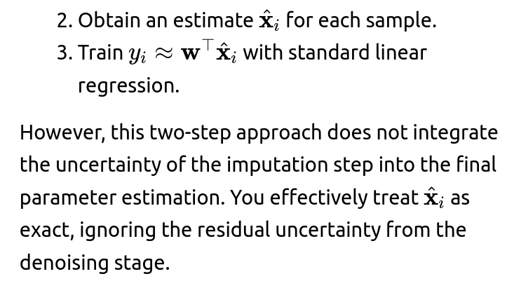
Could we apply data imputation techniques directly to noisy inputs, and then run standard regression?
An alternative to explicitly modeling input noise in the likelihood is to try to “clean” the inputs first, then apply classical regression. For instance, you might:
Use an imputation or denoising algorithm (like a Kalman filter for time-series, or a denoising autoencoder for high-dimensional data).

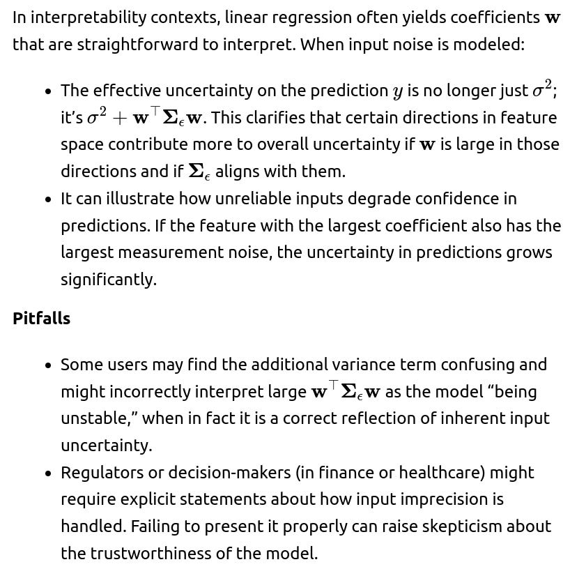
How does the noisy-input formulation help interpret results when explaining the model?

Real-world advantage
Explaining to stakeholders that “due to uncertain measurements in these specific features, our predictions carry an extra margin of error” can make the model’s predictions more believable than a simplistic single-variance approach.
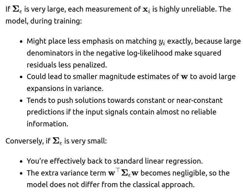
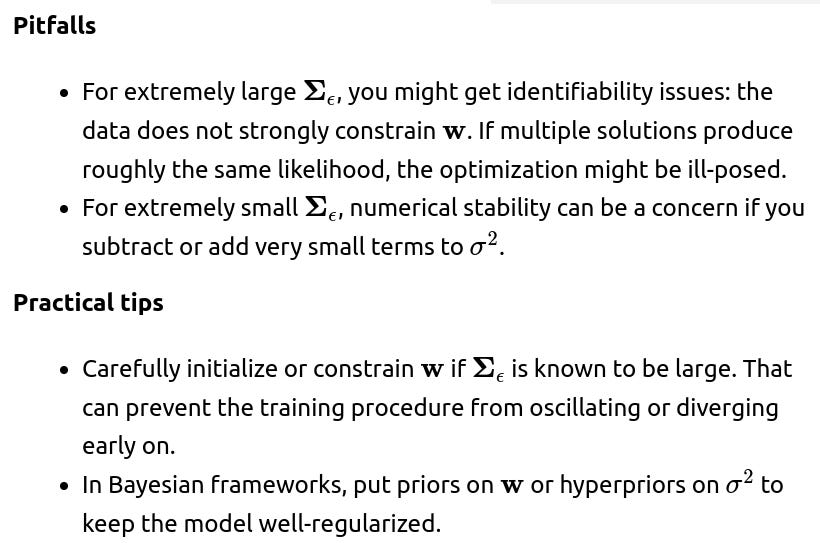
How would you adapt the training procedure if the scale of input noise (Σε) is extremely large or extremely small?

How could you validate that modeling input noise actually improves performance or reliability?
In practice, we want to confirm that the extra complexity of modeling input noise is justified. Some ways to validate:
Held-out or cross-validation: Evaluate predictive performance and calibration of uncertainty. Does the noise-aware model produce more accurate predictions (lower MSE) or more realistic predictive intervals?
Simulations: Generate synthetic data where you know the true input noise distribution. Compare the estimated parameters w^ to ground truth.
Out-of-sample reliability: In real sensor tasks, measure how well the model’s predicted intervals align with new data from sensors. If your model states, “With 95% probability, y is in this band,” check actual coverage frequency.
Pitfalls
If the noise in the real data is not actually as big as hypothesized or if it’s not of the assumed type, the advantage might be small.
Overfitting or tuning too many hyperparameters for the noise model can degrade interpretability and generalization.
Edge scenarios
If your data pipeline cleans or filters inputs heavily before the modeling stage, you might find minimal gains from explicit input-noise modeling.
In critical systems (medical devices, engineering), even modest improvements in uncertainty quantification can be very valuable.
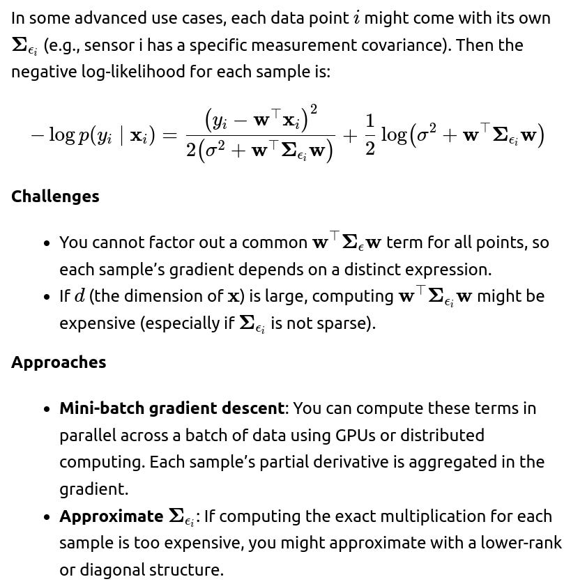
How would you parallelize or scale training if the dimensionality of x is large and each x has its own Σε?

Approximations to the covariance might degrade accuracy if some off-diagonal correlations are critical.
Real-world examples
A large sensor network with thousands of sensors, each with its own measurement reliability profile.
Personalized user data in a recommendation system, where each user has different uncertainty in certain features (demographics, behavior patterns).
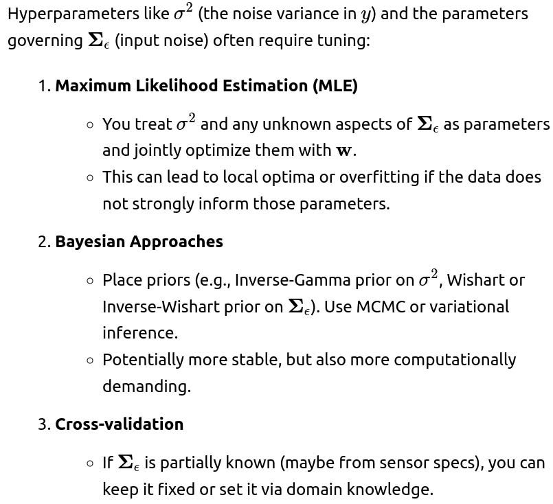
How do you handle hyperparameter tuning for σ² and Σε in practice?