
ML Interview Q Series: Optimal Box Sizing for Defect Control Using Binomial Probability Calculations.

Browse all the Probability Interview Questions here.
A machine produces items of which 1% are defective. How many items can be packed in a box while keeping the chance of one or more defectives in the box to be no more than 0.5? What are the expected value and standard deviation of the number of defectives in a box of that size?
Short Compact solution
Let X be the random variable denoting the number of defectives when n items are put into a box, each item having a 1% probability of being defective independently of the others.
The probability that there are zero defectives is (0.99)^n. Therefore, the probability of at least one defective is 1 – (0.99)^n.
We require 1 – (0.99)^n ≤ 0.5, which simplifies to (0.99)^n ≥ 0.5.
Solving for n gives n < log(0.5) / log(0.99) ≈ 68.97, so n = 68.
With n = 68, the expected value of X is 0.68, and the standard deviation is √(0.68 × 0.99) ≈ 0.82.
Comprehensive Explanation
Deriving the number of items (n)
Consider the number of defective items X in a box of size n. Since each item has a probability p = 0.01 of being defective, X follows a Binomial distribution with parameters n and p.
The probability that there are no defectives (i.e., X = 0) is (1 – p)^n, which in this case is (0.99)^n. Therefore, the probability of having at least one defective (i.e., X ≥ 1) is:

Rearrange this to get:

Taking natural logarithms on both sides:

Because ln(0.99) is a negative number, dividing both sides by ln(0.99) flips the inequality. We ultimately need n to satisfy:
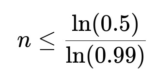
Numerically, ln(0.5) is negative, and ln(0.99) is also negative. Evaluating the fraction yields approximately 68.97. Since n must be an integer, we choose n = 68.
Expected value and standard deviation for the Binomial(n, p)
For a Binomial(n, p) random variable X:
The expected value E(X) = n * p.
The variance Var(X) = n * p * (1 – p).
The standard deviation σ(X) = √(n * p * (1 – p)).
Here, n = 68 and p = 0.01.
Hence,

and

Both of these are intuitive: if only 1% of items are defective, on average we expect 1% of the 68 items (i.e., 0.68 items) to be defective, and the standard deviation measures how much variability we have around that average.
Follow-up questions
1) How would we verify this probability programmatically in Python?
You could write a short Python script that simulates the process many times (Monte Carlo simulation) or directly computes the binomial probability. Below is an example using direct binomial probability from Python’s math library:
import math

# Probability each item is defective
p = 0.01

# Number of items in a box
n = 68

# Probability of zero defectives (using binomial formula or direct approach)
prob_zero_defectives = (1 - p)**n

# Probability of at least one defective
prob_at_least_one = 1 - prob_zero_defectives

print("Probability of at least one defective:", prob_at_least_one)
We expect this probability to be roughly 0.5 (just under or around 0.5, depending on rounding).
2) What if the defect rate p changes?
If p changes, we repeat the same derivation:
Probability that X = 0 is (1 – p)^n.
Probability that X ≥ 1 is 1 – (1 – p)^n.
We want 1 – (1 – p)^n ≤ 0.5, so (1 – p)^n ≥ 0.5.
Solve for n: n ln(1 – p) ≥ ln(0.5).
Hence n ≤ ln(0.5) / ln(1 – p).
Depending on p, n will change accordingly.
3) Could we use a Poisson approximation?
When n is fairly large and p is small, X = number of defectives in n trials can be approximated by a Poisson distribution with mean λ = n * p. For n = 68 and p = 0.01, λ = 0.68, which is indeed small. The Poisson approximation to the probability of zero defectives is e^(−λ). For λ = 0.68, e^(−0.68) ≈ 0.507, which is close to (0.99)^68. This gives a probability of 1 – e^(−0.68) ≈ 0.493 for at least one defective, again consistent with the binomial calculation.
4) What are some practical considerations in real-world manufacturing?
Independence assumption: The binomial model assumes each item is defective independently. If manufacturing defects are correlated (for instance, a machine malfunction that affects many items in a row), the actual probability of defectives could differ.
Variability in defect rate: The 1% defect rate might just be an average over time. In real scenarios, p could fluctuate due to material quality, operator skill, machine calibration, etc.
Safety margins: In many cases, manufacturers require a probability of zero defectives far lower than 50%. They might recast the problem with a stricter threshold or require acceptance sampling plans with set confidence levels.
These are important to mention because in a real production environment, you want to monitor the defect rate over time and validate your assumptions about independence, distribution, and tolerances.
5) How does the choice n = 68 help manage trade-offs in cost and quality?
Larger n means you pack more items per box, which reduces packaging cost per item but increases the chance of containing defectives.
Smaller n means you have more boxes to handle but lowers the probability that a single box has a defective item.
Using this type of analysis helps strike an optimal balance between packaging cost and quality assurance requirements.
Such trade-offs often appear in industrial engineering, supply chain optimization, and risk analysis settings.
These explanations and follow-up discussions should prepare a candidate thoroughly for deeper questioning in a FANG-level interview.