
ML Interview Q Series: Optimal Stocking Under Uncertainty: Calculating Expected Leftover, Shortage, and Stockout Probability.

Browse all the Probability Interview Questions here.
You have to make a one-time business decision how much stock to order to meet a random demand during a single period. The demand is a continuous random variable X with a given probability density f(x). Suppose you decide to order Q units. What is the probability that the initial stock Q will not be enough to meet the demand? What is the expected value of the stock left over at the end of the period? What is the expected value of demand that cannot be satisfied from stock?
where mu is the expected demand, i.e. mu = E(X).
Comprehensive Explanation
Understanding these expressions in detail helps clarify why they make sense from both a probabilistic and a practical standpoint.
Probability that Q units are not enough (P(stockout))
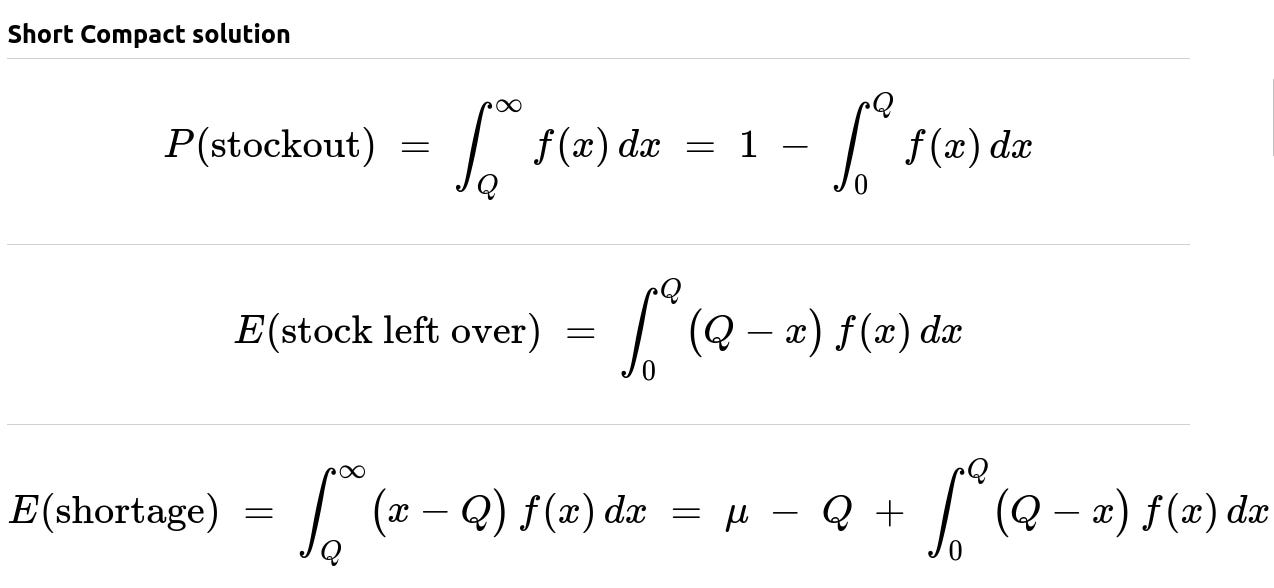
The event that a stockout occurs is exactly the event that X (the random demand) exceeds Q. Since X has a probability density function f(x), the probability of X being greater than Q is the integral from Q to infinity of f(x). Equivalently, it is 1 minus the probability that X is at most Q.
In plain text terms:
P(stockout) = P(X > Q) = integral from Q to infinity of f(x) dx.
Expected stock left over
The quantity of stock remaining at the end of the period is max(Q - X, 0). If demand X is less than Q, there is leftover. If demand X exceeds Q, there is no leftover. By focusing on only those values of x up to Q, one can see that the leftover is Q - x whenever x < Q and 0 when x >= Q. Hence the expected leftover is captured by integrating (Q - x) * f(x) from 0 to Q.
Expected shortage
The shortage (i.e. unmet demand) is the amount by which X exceeds Q if X > Q, and 0 otherwise. Thus it is the random variable max(X - Q, 0). By integrating (x - Q) * f(x) from Q to infinity, one obtains the expected shortage. This can also be rewritten in an alternative form:
E(shortage) = integral from Q to infinity of (x - Q) f(x) dx = mu - Q + integral from 0 to Q of (Q - x) f(x) dx.
An intuitive way to see where mu - Q arises is to recall that the total average demand is mu. Subtracting Q accounts for the fact that some portion of demand is met by the stocked units, but one then adjusts by the portion that is “overcompensated” in scenarios where Q > X.
Why these formulas matter
Probability of stockout gives a direct measure of risk: the higher this probability, the more often one is unable to meet all demand.
Expected leftover is crucial for understanding how much excess stock typically remains unsold or unused. This is extremely relevant in inventory management, where leftover stock might be sold at a discount or represent unsold perishable goods.
Expected shortage captures the average amount of unfilled demand, which can translate to loss of sales or penalty costs if one under-stocks.
Possible Follow-Up Questions
How can we use these expressions to decide the optimal order quantity Q?
One typically introduces cost parameters:
Cost for each unsold unit (overage cost).
Cost for each unit of unmet demand (underage cost).
The classical “newsvendor model” solution balances these costs to arrive at the Q that minimizes the expected total cost. The optimal Q is often given by the critical fractile formula that sets P(X <= Q) = underage_cost / (underage_cost + overage_cost). In practice, you would also look at the distribution function F(x) and solve for the Q that satisfies F(Q) = that ratio.
If the demand distribution were discrete rather than continuous, how would these expressions change?
The same conceptual approach applies, but integrals become sums:
P(stockout) becomes sum over x >= Q of P(X = x).
E(stock left over) becomes sum from x=0 to x=Q-1 of (Q - x)*P(X = x).
E(shortage) becomes sum from x=Q+1 to infinity of (x - Q)*P(X = x).
Could we estimate these integrals when f(x) is unknown?
Yes. In real scenarios, the exact probability density f(x) is often unknown. One might:
Use a parametric approach (e.g. normal, Poisson) and estimate the parameters from data.
Use non-parametric or empirical distribution approaches based on historical demand samples. Then numerical integration or direct sample-based approximations (e.g. Monte Carlo) can give approximate values for these expected quantities.
What happens if Q is very large or very small?
If Q is extremely large, P(stockout) goes to 0, but E(stock left over) might become huge because you will likely stock far more than needed.
If Q is extremely small, P(stockout) goes to nearly 1, but E(stock left over) is almost 0. However, E(shortage) will be large.
How might we simulate this in Python?
Below is a rough snippet showing how to approximate these quantities numerically, assuming we have:
A function
f_pdf(x)that returns f(x), andA function
F_cdf(x)that returns the cumulative distribution.
import numpy as np

def probability_of_stockout(Q, F_cdf):
    return 1.0 - F_cdf(Q)  # Because F_cdf(Q) = integral of f from 0 to Q

def expected_leftover(Q, f_pdf, xmin=0.0, xmax=1000.0, num_points=10**5):
    # Numerical integration for demonstration
    xs = np.linspace(xmin, Q, num_points)
    pdf_values = f_pdf(xs)
    integrand = (Q - xs) * pdf_values
    return np.trapz(integrand, xs)

def expected_shortage(Q, f_pdf, xmax=1000.0, num_points=10**5):
    xs = np.linspace(Q, xmax, num_points)
    pdf_values = f_pdf(xs)
    integrand = (xs - Q) * pdf_values
    return np.trapz(integrand, xs)
In real practice, you would tailor the range of integration and the step size to the distribution at hand and confirm you integrate far enough into the tail so that the probability mass has mostly been covered.
All of these considerations are typical of real interview-level probability and inventory questions. They show both your mastery of the fundamental equations and your knowledge of real-world considerations such as partial information or approximate distribution fits.
Below are additional follow-up questions
How would you handle situations where the demand might be correlated with other products or external factors?
In many real-world scenarios, demand for one product does not occur in isolation. It can be correlated with:
Demand for complementary or substitute products.
Seasonal or temporal factors (e.g., holidays).
Economic indicators or regional variables.
When such correlations exist, straightforward application of a univariate distribution for X might lead to suboptimal decisions because it neglects the information contained in other correlated variables. Here are key considerations:
Joint Demand Modeling: Instead of modeling a single product’s demand independently, you might need a joint distribution model or a regression-based approach to capture the relationship between multiple products or external factors. For instance, if product A’s demand has historically spiked when product B’s demand is high, a univariate approach for A alone might underestimate (or overestimate) A’s tail probabilities.
Multivariate Forecasting: In practice, you might leverage techniques such as Vector Autoregression (VAR), multivariate time-series forecasting, or machine-learning-based forecast models that incorporate data from multiple related features.
Inventory Coordination: If you decide the inventory level of multiple products together (e.g., because of shared storage constraints or shared lead times), the correlation can be used advantageously to hedge risk. For example, higher stock of product A might partially mitigate shortfalls if there’s a possibility to divert resources or if some demand can shift from B to A in certain circumstances.
Pitfalls:
Overlooking correlation can cause you to either under-stock or over-stock if your forecast model doesn’t properly account for large swings in demand caused by external factors.
Overfitting the correlation in a small dataset may create spurious relationships that fail in real operation.
In summary, capturing correlation often involves building more complex probabilistic or machine learning models, but it can yield better alignment between your forecasts and reality.
How does lead time or ordering lag influence these formulas?
In a strict single-period newsvendor framework, the assumption is that you place one order and meet demand over that fixed period. However, in many practical scenarios, there is a lead time between ordering and actually receiving the goods. This creates a few complications:
Demand During Lead Time: If demand can occur while waiting for the stock to arrive, then the effective demand faced by that particular order might be X plus additional random demands that accumulate during lead time. You may need to forecast the total demand from the time the order is placed until the end of the selling period.
Safety Stock Concept: In multi-period contexts with lead times, the well-known formula for safety stock is derived from ensuring a certain service level over the lead-time demand distribution. The single-period approach gets extended to deciding an optimal reorder point: reorder when your inventory drops below some threshold that accounts for the uncertainty in demand over the lead time.
Pitfalls:
Underestimating lead time variability can result in frequent stockouts if lead time is sometimes longer than anticipated.
If lead time is uncertain, the variance of demand over that lead time may be larger, requiring additional buffer.
Relevance to the Single-Period Formulas: The same idea of balancing overage and underage cost remains. But the random variable X that you plug into your newsvendor formula might become “demand over the lead time plus the selling period,” depending on the exact scenario.
Hence, you’d adapt the single-period model by re-defining the time horizon for the random demand to match the entire time from order to period’s end.
What if the demand can be partially fulfilled by multiple orders within the period?
A purely single-period model implies you place exactly one order, then meet demand from that batch. In some industries, you may be able to place multiple orders within the same period if your suppliers can fulfill them quickly. This changes the problem significantly:
Multiple Replenishments: With frequent replenishments, you may hold less initial inventory Q, then replenish as you see real demand materialize. This approach reduces risk of overstocking.
Rolling Horizon Forecast: Each time you reorder, you update your forecast based on the observed demand trend so far. This approach is more dynamic than a single-shot decision.
Different Cost Dynamics: You might pay higher shipping or handling costs for multiple smaller orders, or your supplier might charge more per unit if the order sizes are small. The cost structure could become a more elaborate function of Q.
Pitfalls:
Not having real-time demand data or accurate demand updates can hinder the benefits of multiple orders.
Rapid changes in supplier availability or shipping constraints can negate the ability to “just reorder on the fly.”
In short, the single-period model might not directly apply if repeated orders can be placed. Instead, multi-period inventory models—like base-stock policies—are a better fit.
What if the leftover stock can be sold in a secondary market or used in future periods?
In the classic single-period newsvendor, leftover stock is either worthless or sold at a salvage value. In some real-world settings, leftover inventory from one period might still be useful or can be sold elsewhere. The decision to stock Q now depends on the salvage or carryover strategy:
Salvage Value vs. Next-Period Usage: If leftover stock can be carried forward with minimal cost, the “penalty” for overstocking is much lower, effectively shifting the optimal Q upwards since you’re not stuck with worthless inventory.
Multiple Selling Channels: You might have a secondary market or an online channel to liquidate leftover inventory. The expected leftover cost in that scenario is not just (Q - X) but (Q - X) times some net cost or net revenue factor.
Pitfalls:
Overestimating salvage value can cause systematic overstocking, incurring storage and holding costs that exceed the true salvage benefit.
Markets for leftover goods may be volatile, with uncertain resale prices. This reintroduces an additional random factor that must be modeled.
Hence, in formulas, you would replace the “cost of leftover” with an expected salvage cost or net salvage revenue. That modifies the cost trade-off in your newsvendor solution.
What if the distribution of demand has a high probability of extremely large values (heavy tails)?
In many practical situations—especially with, say, consumer electronics or fashion goods—demand can exhibit a heavy tail. This means the probability of very large demands, while small, is not negligible. If you assume a light-tailed distribution (e.g., normal) in such a scenario, you might not stock enough and can be underestimating P(stockout):
Model Choice: You might need to consider distributions like Pareto, lognormal, or stable distributions to capture extreme demand events.
Risk Management: If one or two “outlier” events can make or break profitability (imagine a viral phenomenon spiking demand unexpectedly), you may want to hold a higher Q as a hedge, or develop more flexible supply chain strategies to handle such surges.
Pitfalls:
Traditional newsvendor solutions based on standard distributions may systematically underestimate inventory levels in the presence of heavy tails, leading to frequent or catastrophic stockouts.
Heavy-tailed distributions can also complicate numerical integration or simulation. You need to ensure you capture the tail behavior accurately (e.g., simulating out to a very high quantile to ensure there is minimal leftover probability mass).
Therefore, a robust approach is to validate your demand distribution modeling assumptions with real data and, if the data exhibits large skewness or kurtosis, adopt or test a model known to handle heavy tails.
How do you handle scenarios where demand can be zero or negative?
In typical business contexts, negative demand does not literally occur. However, some data pipelines might feed returns or cancellations into the demand measure, making the net “demand” appear negative in certain periods if returns exceed sales. Also, demand for new products that fail to sell might effectively result in zero demand. Here’s what to consider:
Zero Demand: If the distribution of X has significant mass at 0, then the integral from 0 to Q to compute leftover still works, because Q - 0 = Q leftover. However, you might want to model P(X=0) distinctly in a mixed distribution or add a point mass to capture that event precisely.
Negative Net Demand: If returns are included, you need a more nuanced approach. Negative “demand” effectively means you’re getting inventory back. In that case, you may want to separate out “gross demand” from “returns,” each with its own distribution, to keep the math more interpretable.
Pitfalls:
Simply ignoring negative demand data or forcing it to zero can bias your estimates of actual demand variability.
Failing to properly account for returns can lead to overestimating net consumption of inventory.
Hence, a better approach is to incorporate a returns process or at least treat negative values separately in modeling. The key is to correctly represent how net inventory changes under returns.
How to handle real-time data updates during the period for better decisions?
In some businesses (e.g., e-commerce with real-time analytics), you may observe part of the demand as it happens and still have time to adjust Q:
Bayesian Updating: You can incorporate real-time sales data to update your demand distribution parameters. For example, if halfway through the period you see that demand is trending higher than forecast, you might place an emergency order if lead times permit.
Adaptive Strategies: Machine learning models can continuously refine the forecast as new data arrives.
Pitfalls:
Lead times might still be too long to benefit from mid-period insights.
Overreacting to short-term signals may introduce instability in ordering patterns (the “bullwhip effect” in supply chains).
Thus, if mid-period corrections are possible, the single-period newsvendor approach merges into a rolling-horizon or dynamic inventory control model, which is more complex but can better leverage incoming demand information.
Can these formulas be extended to account for random yields or defective stock?
Another layer of complexity arises if the supplier’s yield is uncertain. For instance, you order Q units, but only a random fraction arrives in good condition:
Effective Q: Let Y be the random yield. Then the “usable” quantity is min(Y, Q) if yield is bounded by the order, or sometimes Y can exceed Q if the yield is proportion-based.
Distribution Overlap: Now the shortage event depends not just on X > Q but also on Y < Q. Specifically, the shortage is max(X - Y, 0). You would then need a joint distribution for X (demand) and Y (yield), or at least an assumption about whether X and Y are independent.
Pitfalls:
Treating yield as deterministic can lead to systematic understocking if yield is typically below Q.
If yield depends on external factors also correlated with demand, you get a complicated multi-variance scenario requiring more advanced models.
Hence, while the original formula can still be adapted to incorporate E[max(X - Y, 0)], the modeling complexity goes up significantly because you need a distribution for Y and possibly for the correlation between X and Y.
What if there's a penalty or goodwill loss when shortage occurs?
In many industries, failing to meet demand can cause more than just immediate loss of sales. It might lead to reputational damage, loss of future customer loyalty, or contractual penalties. This changes the cost structure:
Incorporate Penalty Costs: Instead of purely evaluating lost profit from unfilled demand, you add a penalty term that might scale with the magnitude of the shortage or might be triggered once any shortage occurs (binary penalty).
Probability of Stockout: If there is a severe penalty for even a single shortage event, it might be rational to choose a Q that makes P(stockout) extremely small, even if that results in more leftover on average.
Pitfalls:
Overestimating penalty costs leads to unnecessarily large inventory levels, tying up capital and incurring holding or obsolescence risk.
Some penalty costs are intangible or hard to quantify, such as reputation damage. Overly simplistic assumptions can misrepresent the true trade-offs.
Thus, you might incorporate a more nuanced cost function that includes intangible or long-term impacts, which modifies the “optimal” Q found by classical newsvendor analysis.
How do you decide a distribution to model demand when you only have a small dataset?
A major challenge in real businesses is limited historical data or data that spans an atypical period (like recent disruptions). Modeling demand with insufficient data involves:
Parametric vs. Non-Parametric:
Parametric: Fit a known distribution (e.g., Poisson, normal) but risk mis-specification if the distribution doesn’t match the real demand shape.
Non-parametric (e.g., kernel density, bootstrapping): May better fit the observed data distribution but can be unstable if data is sparse or if demands outside your sample range can occur in real life.
Bayesian Approaches: You could impose a prior distribution on parameters (e.g., a Gamma prior for Poisson demand) and update them with your limited data, hopefully gaining a more robust estimate of the demand distribution.
Pitfalls:
Overfitting: Relying too heavily on a small sample might lead you to a very narrow demand forecast that ignores the possibility of extreme events.
Underfitting: Conversely, you might pick a broad distribution that doesn’t capture useful structure, leading to large uncertainty in your Q decision.
Therefore, you must balance parsimony with realism. Often, domain knowledge or combining small historical samples with expert forecasts can mitigate data constraints.
How do continuous improvements or data re-collection efforts help refine Q in future periods?
Even in a single-period setting, you might experience multiple distinct single-period events over time (e.g., monthly product releases). Each event is “single period,” but over many such cycles you can refine:
Learning from Past Orders: After each cycle, record actual demand X, leftover Q - X (if any), and shortage X - Q (if that’s positive). This data helps you update your distribution or parameters.
Iterative Parameter Tuning: If you’re using a parametric approach, adjust parameters (mean, variance) after each cycle to capture shifts in consumer tastes, seasonal effects, or economic changes.
Pitfalls:
Changes in consumer behavior over time might invalidate older data.
Demand distributions can shift unpredictably (e.g., due to new competition), so you need continuous model recalibration.
Hence, although each single period stands on its own for the ordering decision, you gain valuable information from each repetition that can improve your future single-period outcomes.