
ML Interview Q Series: Optimizing Buffer Emptying Costs for Poisson Arrivals using Regenerative Process Theory.

Browse all the Probability Interview Questions here.
14E-11. Messages arriving at a communication channel according to a Poisson process with rate λ are temporarily stored in a buffer with ample capacity. The buffer is emptied every T time units, where T>0 is fixed. There is a fixed cost of K>0 for emptying the buffer. A holding cost at rate h>0 per unit time is incurred for each message in the buffer. Identify a regenerative stochastic process and find the long-run average cost per unit time as a function of T. What value of T minimizes the long-run average cost per unit time?
Short Compact solution
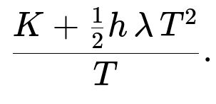
One can define a “cycle” as the time interval between two successive buffer-emptying events. Because arrivals follow a Poisson process (memoryless property), these emptying epochs serve as regeneration points. In each cycle of length T, the expected total cost is composed of a fixed cost K plus the expected holding cost, which turns out to be (1/2) h λ T². Hence, the total cost per cycle is K + (1/2) h λ T². By the renewal reward theorem, the long-run average cost per unit time is
Minimizing this expression in T yields

Comprehensive Explanation
Identifying the Regenerative Process
The key to solving this problem is recognizing that the stochastic process X(t), which denotes the number of messages in the buffer at time t, is regenerative at the epochs when the buffer is emptied. Specifically:
Because messages arrive according to a Poisson process, the number of arrivals in any interval is independent of the number of arrivals before that interval.
Emptying the buffer at time multiples of T effectively “resets” the system to an empty state.
These reset times are regeneration points: the process restarts statistically at each of these empty times.
Defining a Cycle and Applying Renewal Reward
We look at one “cycle” of length T, starting immediately after the buffer is emptied and ending right before the next emptying:
Over this cycle, we pay a fixed emptying cost K exactly once (at the end/beginning of the cycle).
Arrivals accumulate in the buffer, incurring a holding cost at rate h for each unit time that each message stays in the buffer. Since the arrival process is Poisson with rate λ, the expected number of arrivals over the interval [0, T] is λT.
To compute the expected holding cost, we note that the arrival times within a cycle are (by memorylessness and order statistics of the Poisson process) equivalent to T i.i.d. exponential interarrival times with parameter λ, or equivalently viewed via Erlang/Gamma distributions for the nth arrival. In simpler terms:
The average time a message stays in the buffer before it is removed is (T – x), where x is the arrival time of a message within the cycle.
By integrating or using well-known results on the expected waiting time of arrivals within a fixed interval, one obtains the expected total holding cost in the interval to be (1/2) h λ T².
Hence, the expected cost in one cycle of length T is:
Fixed cost: K
Holding cost: (1/2) h λ T²
Long-Run Average Cost
By the renewal reward (or renewal cost) theorem, the long-run average cost per unit time is the expected cost per cycle divided by the expected cycle length. The cycle length is T, so the average cost rate C(T) is

We can split it out as:
K / T
plus (1/2) h λ T
Minimizing the Cost Function
To find the optimal T that minimizes C(T), we take the derivative of C(T) with respect to T and set it to 0 (and confirm it is indeed a minimum by second derivative or by convexity arguments). Solving this straightforward calculus problem yields:

This T* gives the best balance between incurring too many fixed emptying costs (if T is too small) and too much holding cost (if T is too large).
Potential Follow-up Questions
Why is the process considered regenerative precisely at the buffer-emptying epochs?
In a Poisson arrival process, the “memoryless” property ensures that the future evolution (i.e., new arrivals and so forth) does not depend on what happened before a complete reset. When we empty the buffer at time multiples of T, we return to a state of zero messages in the buffer, and from that point onward, the arrival process starts afresh (still Poisson with rate λ). This property is exactly what defines regeneration: after an emptying event, the system probabilistically behaves as it did at time zero.
Can we explain intuitively why the holding cost is proportional to T²?
Over the interval [0, T], on average, λT messages arrive. If arrivals were uniformly distributed on [0, T], each arrival would stay in the buffer for an average duration of about T/2, leading to an intuitive holding cost ∝ (number of arrivals) × (average waiting time) = (λT) × (T/2) = (λ T²)/2. A more precise derivation integrates (T–x) over the arrival time distribution, but the result is consistent with this simple reasoning.
What happens if T → 0?
If T approaches 0, we are emptying the buffer extremely frequently. That drives the cost K/T to become enormous because we pay the emptying cost K almost continuously. Although the holding cost (1/2) h λ T tends to 0, the term K/T dominates, making the total cost per unit time very high.
What if T → ∞?
If T becomes extremely large, we pay the fixed cost K less frequently. But each message is kept in the buffer for nearly the full time T (on average around T/2), leading to a huge holding cost. So the (1/2) h λ T term dominates, again driving the cost per unit time upward.
Could the optimal T be any local maximum or inflection point?
No. By inspecting the derivative carefully, you see the cost function is convex in T > 0 (because one term is inversely proportional to T and the other is linear in T). This means that the point you get from setting the derivative to zero is indeed a global minimum, not a local maximum or an inflection point.
How do we implement this in a practical system?
In many real systems, you might estimate λ (the arrival rate) and h (the holding cost rate) empirically. For instance, you could track the average traffic intensity (arrivals per second) and place a nominal monetary value on holding a message in the buffer (e.g., h). Then measure your overhead or cost K for emptying the buffer (this could be CPU overhead, energy consumption, or actual monetary cost). Once these parameters are estimated, you would set T to sqrt(2K/(h λ)) in real-time or at design time for best steady-state cost efficiency.
How would randomness in T or additional constraints (like a maximum queue length) affect the analysis?
If T itself were random (say we empty the buffer at random intervals with some distribution), you would need a different renewal analysis where the cycle length is a random variable. The same principles apply, but you have to compute the expected cycle length and expected cost per cycle under that new distribution.
If there is a finite buffer or a constraint on maximum waiting time, that might force more frequent emptying or lead to a queue-overflow policy. Those modifications lead to more complex cost equations and might require different analyses, but the same renewal concepts often still apply, provided you identify the correct regeneration points.
These considerations are typical in queueing and cost optimization problems and reflect real-world complexities where exact uniform emptying times are not always feasible. The essential principle remains that balancing fixed overhead costs with the rising holding costs in a backlog is often the key to an optimal strategy.
Below are additional follow-up questions
What if the arrival rate λ is not constant over time but instead time-varying?
When λ changes with time (for instance, λ = λ(t) with peak and off-peak periods), the assumption of a stationary Poisson process no longer holds. In a nonstationary Poisson process, the rate function λ(t) varies over the day or operating cycle.
Analysis Complexity: The expected number of arrivals in an interval [0, T] is then the integral of λ(t) over that interval, and the distribution of arrival times is more involved than in the stationary Poisson case. This complicates deriving an exact closed-form expression for the expected holding cost. We generally need to compute
(expected cost per cycle) = fixed cost K + integral over 0 to T of (h times the expected number of messages in buffer at each instant).
Heuristic Approaches: One might approximate or bound the cost by looking at average arrival rate (say, an average λ̄) over the period. Then we can do a near-optimal design: T* ~ sqrt(2K / (h λ̄)). But in reality, if λ(t) is highly variable, it might be optimal to empty more frequently during peak times and less frequently during off-peak times, leading to a more intricate policy than a single constant T.
Piecewise-Stationary Approximation: In practice, one might split the timeline into segments where λ is roughly constant and compute a local T for each segment. However, switching costs between different T schedules might arise, making the analysis more nuanced.
How does the analysis change if K, the cost of emptying the buffer, itself is stochastic?
If K is not a constant but a random variable (say, K depends on various factors like system load, or the cost of triggers at certain times of day fluctuates), then each cycle might incur a different emptying cost K_i.
Regenerative Structure: The process is still regenerative at emptying epochs, but now the expected cost per cycle is E[K] + (1/2) h λ T² (assuming the holding cost derivation remains the same).
Variance and Risk: If K is random with an expectation E[K], simply plugging E[K] into the average cost formula might suffice for the mean cost minimization. If we care about cost variability or risk, we might want to incorporate a penalty or risk measure (e.g., a cost variance term) that complicates the objective function beyond just E[K].
Practical Implementation: In a real system, we might estimate E[K] from historical data. If the distribution is stable, E[K] is a good approximation. If K can be extremely large in certain states (heavy load), a more robust or conservative policy might set T to reduce the chance of incurring that large cost.
Could we employ a partial-emptying policy within each cycle, and how would that affect the cost?
Instead of emptying the entire buffer only at time T, one might consider partially emptying it at intermediate times, then completely emptying at T.
Impact on Cost: Each partial emptying could have its own fixed or variable cost, changing the cost structure. The expected holding cost might reduce because some messages are removed earlier, but the overhead from partial emptying events might raise K or lead to multiple smaller K-like charges.
Complexity: The process might lose a simple renewal structure if we are not returning to an empty buffer at the partial-empty events. The system might only be strictly regenerative at the times of complete emptying, so the cost analysis is more complicated.
Optimal Strategy: Typically, in classical queueing theory with a simple fixed cost K per “batch removal,” a single emptying event per cycle is still optimal if that cost K does not change with the number of partial empties. But real-world systems might have a discounted cost for partial empties or might tie cost to batch size, creating a more complex optimization.
If arrivals can happen in batches instead of one by one, does that change the holding cost derivation?
In certain applications, messages (or jobs) might arrive in bursts. For instance, you might have a compound Poisson process where each arrival event brings a random batch of messages.
Batch Size Distribution: Let M be the random batch size with mean E[M]. Then in an interval [0, T], the total number of messages arriving is approximately the sum of batch sizes over the number of batch arrivals. If the batch arrivals themselves follow a Poisson process with rate λ, then the expected total messages in [0, T] is λT × E[M].
Holding Time: The average waiting time for any one arrival in that interval is still about T/2 (assuming uniform arrival over [0, T]), so the expected holding cost becomes about h × ( (λT E[M]) × (T/2) ) = (1/2) h λ E[M] T².
Conclusion: Many times the batch arrival model just modifies the effective arrival rate by a factor of E[M]. The formula for T* becomes sqrt(2K / (h λ E[M])) if everything else is the same. The fundamental renewal argument still stands.
What if there is a capacity limit on the buffer, or blocking occurs when the buffer is full?
So far, we assumed an “ample capacity” buffer. In a real system, the buffer might have limited space. If it fills up, new arrivals may be lost or blocked.
Non-Empty Cycles: The system might still be regenerative at empties, but the state space is more complicated because the process can hit maximum capacity prior to T. The cost structure might need to account for lost messages or penalty for blocking.
Analytical Challenge: The arrival process still runs, but once the buffer hits capacity, arrivals that occur before the next emptying time are discarded (or queued elsewhere). The expected holding cost might be smaller (since fewer messages are held), but you might incur a penalty for lost traffic or missed jobs.
Optimal T Trade-Off: With blocking, making T too large can cause many arrivals to be lost if the buffer saturates early in the interval. That might impose a high “loss penalty” if losing messages is costly. As a result, you might want to shorten T to reduce blocking. The mathematics become more involved, often requiring either Markov chain models or approximate queueing analysis.
What if the cost rate h is itself a function of time or the number of messages in the buffer?
In some real scenarios, the holding cost could escalate as the buffer grows (maybe each additional message imposes an incremental resource cost). Then h is no longer a constant but h(n) depends on n, the number of messages in the buffer, or h(t) changes over time.
Dependence on n: If h(n) is higher for larger n, the holding cost integrates a function of how many messages are in the queue at each instant. This might make the cost structure more complicated but can still be tackled by summing up the expected time that the process spends with i messages in the system (i from 1 to n).
Dependence on t: If h(t) changes with time (e.g., cost is higher during peak hours), then you can attempt to do a piecewise integral of h(t) times the expected queue length at t. The analysis still uses renewal arguments, but the formula for the expected cost per cycle might no longer have a simple closed form.
Possible Mitigation: A system might choose a shorter T in intervals where h(t) is high to reduce the high holding costs, but let T be larger when h(t) is low. That leads to a time-varying emptying schedule, again complicating the renewal framework unless you treat each cycle as a specialized period with known cost.
Would the approach differ if instead of a fixed T, we use a policy that empties the buffer when it reaches a certain number of messages?
This shifts from a time-based to a state-based (or level-based) policy, often called an M/M/1-type approach with a threshold for service.
Different Regeneration: Now the system “resets” each time the buffer size hits some threshold or we decide to drain it based on queue length. The regeneration points are no longer every T units of time but at random times triggered by the buffer reaching a certain capacity or threshold.
Cost Function: The cost might be redefined. Instead of focusing on T, you focus on the threshold for the queue length. The expected cycle time from empty to threshold becomes a random variable that depends on the arrival process and the threshold. The fixed cost K is incurred each time we flush the buffer. The holding cost is integrated over the random cycle.
Analysis Tools: One typically uses embedded Markov chains or more advanced queueing theory to derive the cycle distributions under a threshold policy. The same principle of renewal reward applies, but the expressions are different.
How does correlation between arrivals or bursty traffic (e.g., Markov-modulated Poisson process) affect the conclusion?
In a Markov-modulated Poisson process (MMPP), the arrival rate itself jumps among different states. This leads to correlation or burstiness in the arrival stream.
Loss of Simplicity: The basic memoryless property that simplifies the regeneration argument no longer strictly holds in the same simple way. If the rate state is not reset at an emptying epoch, the process might not be perfectly regenerative.
Approximate or Extended Methods: In some cases, the system might still be “semi-regenerative” at empty times, but you must track the underlying Markov chain state for the arrival process. The expected cost per cycle depends on the stationary distribution of that chain at the emptying epochs. Detailed computations often involve advanced matrix-analytic methods.
High-Level Lesson: The intuition behind balancing fixed costs K and holding costs still applies, but deriving T* in closed form may not be possible. Practitioners might resort to numerical simulation or approximations.
If the cost of emptying grows with the number of messages, how does that modify the solution?
Sometimes removing a larger queue is costlier than removing a smaller one. For instance, if it takes time or extra resources to process each message. Then the cost to empty the buffer might be K + cN, where N is the number of messages.
Expected Number of Messages: The expected number of messages at the time of emptying is approximately λT, so the emptying cost for each cycle becomes K + c λT.
Total Cycle Cost: Summing up, you have (K + c λT) + (1/2) h λ T² for each cycle.
Average Cost Per Unit Time: ( [K + c λT] + (1/2) h λ T² ) / T = K/T + c λ + (1/2) h λ T.
Optimization: If you differentiate that w.r.t. T, you get a linear function in T plus a term -K/T² from K/T. The result is still straightforward to optimize, but the optimal T shifts due to the extra term c λ. Specifically, you get a new T* that balances the derivative of (1/2) h λ T with K/T². The new formula might be T* = sqrt(2K/(h λ)) just as before, but the presence of c λ in the cost expression can lead to an additional offset or cause you to reevaluate whether T is even optimal or if continuous draining is better.
Does the formula still hold if we only pay the holding cost until the buffer is flushed, but flushing itself also takes time?
If flushing (emptying) the buffer is not instantaneous but takes some duration that depends on how many messages must be cleared, then:
Cycle Length: The length of each cycle might be T + (time to empty). The process is truly regenerated only after the emptying finishes. This extension shifts the renewal interval from T to T + E[emptying time].
Cost Implication: During the emptying time, new arrivals might be blocked or delayed, or in some designs, they might keep arriving. The cost structure might reflect that during the emptying period you have reduced or no buffer occupancy, or if arrivals are blocked, you might face lost demand.
Derivation: The renewal reward theorem still applies, but you must carefully define the renewal cycle, incorporate the expected emptying duration, and any associated cost or lost opportunity. The straightforward T-based formula changes because the denominator in average cost is no longer T but T plus the average flush time.