ML Interview Q Series: Optimizing Models with Latent Variables Using Expectation-Maximization (EM)

📚 Browse the full ML Interview series here.

38. What is Expectation-Maximization (EM) and when is it useful? Describe the setup algorithmically with formulas.

EM is a powerful optimization approach used when data is partially observable or has latent (hidden) variables. It is most commonly applied in scenarios where directly maximizing the likelihood (or posterior) of observed data is difficult due to unobserved or missing variables. A typical example is fitting Gaussian Mixture Models (GMMs), where each observed data point is generated from one of several Gaussian components, but the component “assignment” is hidden.

EM iteratively improves parameter estimates by alternating between an Expectation step (E-step) and a Maximization step (M-step). In the E-step, it computes the posterior distribution of latent variables given the observed data and the current parameter estimates. In the M-step, it re-estimates the parameters by maximizing a surrogate lower bound on the log-likelihood that relies on the distribution computed in the E-step. These two steps are repeated until convergence to a local optimum.

When data is incomplete, or the problem involves hidden variables that make direct maximization intractable, EM can help decompose the objective in a way that iterates toward better parameter estimates.

Detailed Explanation of the EM Setup

Setting and Notation

Suppose you have observed data X and hidden variables Z. The model is parameterized by some parameter set θ. The log-likelihood of the observed data is

It is often very challenging to directly optimize this expression with respect to θ because of the summation (or integration) over hidden variables Z. Instead, EM tackles this iteratively by creating and then maximizing a lower bound on this log-likelihood.

E-step (Expectation step)

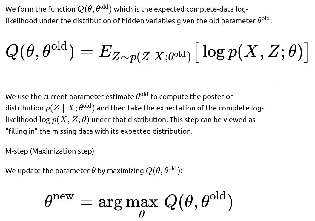
This step uses the “completed” data from the E-step (in a probabilistic sense) to find the best new parameter estimate. The combination of these two steps leads to a monotonic increase in the observed-data log-likelihood (or at least it will not decrease). The process is repeated until θ converges to a (local) optimum.

Why It Is Useful

Directly maximizing log⁡p(X;θ) can be intractable if Z is complicated to sum over or if the integrals are high-dimensional. By splitting the optimization into these two steps, EM offers a systematic way to deal with latent structure. Real-world problems often have missing data or unobserved categories (e.g., mixture models, hidden Markov models, incomplete observation scenarios), so EM is an elegant solution for parameter inference in such settings.

Example: EM for Gaussian Mixture Model

E-step: Compute the responsibilities (the posterior probabilities that each mixture component generated each data point) using the current parameters.

M-step: Re-estimate the means, covariances, and mixing coefficients of the Gaussians to maximize the expected complete-data log-likelihood under those responsibilities.

Because the latent assignments are never directly observed, the EM algorithm’s repeated re-evaluation of these responsibilities is precisely what allows one to fit the mixture model effectively.

Subtleties and Convergence Properties

EM guarantees that each iteration will not decrease the observed-data log-likelihood. But it does not guarantee convergence to a global optimum; it often finds a local maximum dependent on initialization. Careful initialization strategies, restarts with different random seeds, and model selection considerations (e.g., the number of mixture components) can mitigate local optima risks.

Implementation Sketch in Python for a Simple GMM

import numpy as np

def initialize_parameters(X, K):
    n_samples, n_features = X.shape
    means = X[np.random.choice(n_samples, K, replace=False)]
    covariances = [np.eye(n_features) for _ in range(K)]
    mixing_coeffs = np.ones(K) / K
    return means, covariances, mixing_coeffs

def gaussian_pdf(x, mean, cov):
    n_features = len(x)
    norm_const = 1.0 / (np.sqrt((2*np.pi)**n_features * np.linalg.det(cov)))
    x_minus_mean = x - mean
    return norm_const * np.exp(-0.5 * x_minus_mean.T @ np.linalg.inv(cov) @ x_minus_mean)

def e_step(X, means, covariances, mixing_coeffs):
    K = len(means)
    n_samples = len(X)
    resp = np.zeros((n_samples, K))
    for i in range(n_samples):
        for k in range(K):
            resp[i, k] = mixing_coeffs[k] * gaussian_pdf(X[i], means[k], covariances[k])
        resp[i, :] /= np.sum(resp[i, :])  # Normalize responsibilities
    return resp

def m_step(X, resp):
    n_samples, n_features = X.shape
    K = resp.shape[1]
    means = np.zeros((K, n_features))
    covariances = []
    mixing_coeffs = np.zeros(K)

    for k in range(K):
        Nk = np.sum(resp[:, k])
        means[k] = np.sum(resp[:, k].reshape(-1, 1) * X, axis=0) / Nk
        cov_k = np.zeros((n_features, n_features))
        for i in range(n_samples):
            diff = (X[i] - means[k]).reshape(-1, 1)
            cov_k += resp[i, k] * (diff @ diff.T)
        cov_k /= Nk
        covariances.append(cov_k)
        mixing_coeffs[k] = Nk / n_samples
    return means, covariances, mixing_coeffs

def gmm_em(X, K, max_iter=100, tol=1e-6):
    means, covariances, mixing_coeffs = initialize_parameters(X, K)
    log_likelihood = 0
    for _ in range(max_iter):
        resp = e_step(X, means, covariances, mixing_coeffs)
        means, covariances, mixing_coeffs = m_step(X, resp)
        # Optional: compute log-likelihood for monitoring convergence
        # You can break early if improvement is below tolerance
    return means, covariances, mixing_coeffs

Use Cases

EM is used in fitting mixture models, clustering with partial labels, hidden Markov models, factor analysis, and incomplete-data problems where some variables are unobserved. Its strength is in providing a tractable iterative approach when direct optimization of the marginal likelihood is difficult.

Potential Pitfalls

There can be numerical instabilities (like very small or nearly singular covariances). One might need regularization or constraints to stabilize updates (e.g., adding a small constant on the diagonal of covariance matrices). Local optima can be mitigated by multiple restarts. Convergence speed can vary depending on the shape of the likelihood landscape.

Below are potential follow-up questions that often arise in advanced technical interviews, especially in large tech companies, along with thorough discussions of each.

How does EM guarantee that the observed-data log-likelihood does not decrease after each iteration?

Is the EM algorithm guaranteed to converge to the global optimum?

EM generally converges to a stationary point of the observed-data log-likelihood function, but not necessarily the global optimum. It is a coordinate ascent-like method on the evidence lower bound (ELBO). Because many real-world log-likelihood surfaces are non-convex, there might be multiple local maxima. Different random initializations or specialized initialization methods (e.g., K-means for GMM parameters) are often used to search for better maxima. In practice, it converges to a local maximum that is heavily dependent on the starting point.

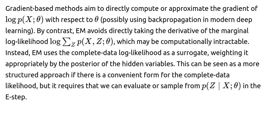
What is the difference between EM and gradient-based optimization methods?

How does EM handle missing data?

When some observations in X are missing, we can treat the missing portions as latent variables. We then proceed with the standard EM approach: the E-step involves computing the distribution over missing values given the observed ones and the current parameters. The M-step updates the parameters by maximizing the expected complete-data log-likelihood. This is often used in situations where data is not fully observed due to sensor failures, incomplete surveys, or any scenario of partial data availability.

Can you explain how EM is used in Hidden Markov Models?

In Hidden Markov Models (HMMs), the observed data are the emissions and the latent variables are the hidden states at each time step. The forward-backward algorithm plays the role of the E-step by computing the posterior distribution over hidden state sequences given the observed sequence and current model parameters. The M-step then re-estimates the transition probabilities, emission probabilities, and possibly initial state probabilities by maximizing the expected complete-data log-likelihood. This specific case of the EM algorithm is often referred to as the Baum-Welch algorithm.

In what ways can we speed up or scale EM for large datasets?

For very large datasets, you can use stochastic approximations, sometimes called Stochastic EM or online EM, where you process mini-batches of data in the E-step to obtain an approximate posterior over hidden variables. Then you update parameters in a manner analogous to stochastic gradient ascent, repeating these partial E and M steps. Variational inference methods can also be seen as generalizations or alternatives to EM in large-scale probabilistic models.

Could we interpret K-Means as a special case of EM?

Yes, K-Means can be seen as a special case of EM for Gaussian Mixtures with the assumption that each Gaussian has an identity covariance matrix and the mixing coefficients are fixed. In that simplified scenario, the E-step of assigning cluster membership based on minimum squared distance can be interpreted as computing posterior responsibilities that collapse to 0 or 1. The M-step of recalculating means is then the standard K-Means centroid update. However, the typical K-Means update rule is a hard assignment, whereas general EM for GMM is a soft assignment (posterior distribution over clusters).

How do you choose the number of components in a mixture model when using EM?

One common approach is to run EM for different numbers of components and then compare the models using model selection criteria such as the Bayesian Information Criterion (BIC) or the Akaike Information Criterion (AIC). These criteria penalize model complexity (i.e., the number of parameters) in addition to evaluating fit on the observed data. Cross-validation can also be employed, though it is more computationally expensive.

How do you handle singularities or degeneracies in Gaussian Mixture Models using EM?

EM updates can cause singularities if a covariance matrix collapses to nearly zero determinant. This typically happens when a cluster collapses to one or very few data points, leading to extremely high likelihood for those data points. Practical ways to mitigate this include putting a small regularization term on the diagonal of covariance matrices during the M-step or setting a minimum cluster size requirement. You can also remove components that have become “empty” (no data assigned) and re-initialize them.

When do you use EM instead of simpler methods or direct gradient-based optimization?

EM is particularly advantageous if you have a well-defined latent variable model where the complete-data log-likelihood is easier to optimize, or if there is a known standard procedure for computing the posterior over latent variables. If the model does not factorize nicely and computing the E-step is as hard as the original problem, direct gradient-based optimization might be preferable. But when the model structure allows relatively straightforward E and M steps, EM can be extremely efficient.

What is the computational cost of EM?

The cost depends on both the E-step and M-step. For Gaussian Mixture Models, the E-step involves evaluating each data point against each mixture component, often O(n×K) where n is the number of data points and K is the number of components. The M-step can involve inverting covariance matrices or summing over data points again. One must carefully manage memory and compute resources for large n or K. For more complex latent variable models, the forward-backward algorithm in HMMs or more advanced inference methods can introduce additional overhead.

If EM guarantees a non-decreasing log-likelihood, why might it get stuck?

It can get stuck in local maxima. The guarantee that EM does not decrease the observed-data log-likelihood only ensures that if the parameter space has multiple local maxima, the algorithm might converge to any of them. This is why multiple initializations or good heuristic or domain-specific initialization strategies are important. Another issue is saddle points, though in practice local maxima are the main concern.

How do you evaluate the quality of an EM-based model after training?

You can compute the final log-likelihood on the training dataset, but that does not directly account for overfitting or the complexity of the model. Model selection criteria like BIC or AIC or cross-validation-based log-likelihood on a held-out validation set are common ways to evaluate the model’s generalization and decide on hyperparameters like the number of mixture components. You can also visualize cluster assignments or responsibilities if the dimensionality is small enough or if you apply dimensionality reduction.

How does EM compare to Variational Inference?

How to deal with non-conjugate models in EM?

Can EM be used for Maximum A Posteriori (MAP) estimation instead of MLE?

Does the order in which we process data in the E-step matter?

In the classical EM formulation, the E-step is typically carried out as a complete pass over the entire dataset to compute or approximate the posterior distribution of all latent variables. The order of data points in that pass does not matter for the final outcome of the E-step because it relies on summations or expectations across all samples. In contrast, if you do a “stochastic” or “online” variant of EM, then you might process mini-batches or single data points in an online manner. The specific strategy in that scenario can slightly change how quickly you converge, but the standard batch EM sees all data for each E-step.

Are there scenarios where EM is less favorable?

If the posterior over latent variables is very difficult to compute or approximate, EM might not simplify the problem much compared to direct likelihood maximization. Also, if each M-step is complicated to perform or if the model structure does not admit closed-form solutions, you might have to use specialized or approximate methods for both E and M steps, which can diminish the advantages of EM. Another scenario is if you can compute the gradient of your marginal likelihood directly and if you prefer using advanced optimization methods (e.g., second-order gradient methods). In that case, a direct optimization approach might be more straightforward.

Is EM related to the Minorize-Maximize (MM) principle?

How does EM behave if the model is misspecified?

EM tries to maximize the likelihood under the assumed model. If the true data generating process significantly differs from your model assumptions (e.g., wrong distributional assumptions, missing important variables), EM might converge to a poor local optimum or yield biased estimates. Model misspecification is a broader issue than just the choice of the inference algorithm, but EM will still converge to the best parameters under the incorrect model, rather than revealing that the model is inadequate. Goodness-of-fit tests, model diagnostics, or alternative modeling approaches might be necessary.

How do we implement Early Stopping in EM?

In practice, you can monitor the change in the observed-data log-likelihood across iterations. If the increment falls below a small threshold, you can stop. This threshold-based stopping is akin to early stopping in gradient-based methods, though typically in EM you are monitoring “lack of improvement” rather than overfitting. Another approach is to evaluate a separate validation set log-likelihood and stop if it deteriorates or no longer improves. However, classical EM does not have an overfitting mechanism the same way neural networks do, so standard practice is usually to iterate until convergence or a maximum iteration limit.

---

Below are additional follow-up questions

What are the “complete-data” and “incomplete-data” viewpoints in EM, and how do they differ conceptually?

In EM, the central idea is that we have data with missing or latent components. From a conceptual standpoint, “complete data” refers to the dataset that would be available if all variables—both observed and latent—were known. “Incomplete data” refers to the real-world situation in which only the observed portion is available, while the latent variables remain hidden. The complete-data log-likelihood is typically simpler to work with, because it assumes access to all variables. However, in reality, we cannot directly write down or maximize this quantity due to the missing pieces.

EM bridges this gap by alternately:

1. “Completing” the data probabilistically (the E-step), using the conditional distribution of latent variables given the observed data and the current parameter estimate.

2. Optimizing model parameters based on the expected complete-data log-likelihood (the M-step).

A subtle but important conceptual distinction is that in the complete-data perspective, we treat the latent variables as known for the sake of computing a simpler likelihood function, while in the incomplete-data perspective, we face the challenges of marginalizing over these unknowns. This difference arises frequently in real-world scenarios with partial observations, sensor failures, or inherently hidden states (e.g., mixture components). By toggling between these viewpoints during each iteration, EM circumvents the direct maximization of the intractable marginal likelihood and converges to parameters that locally maximize the observed-data likelihood.

Pitfalls and Edge Cases:

• If the definition of the complete-data log-likelihood is incorrect or fails to capture constraints on the latent variables, the EM algorithm can produce nonsensical parameter updates or fail to converge.

• In some models, specifying the complete-data likelihood might introduce additional hyperparameters that need to be calibrated, further complicating the E-step or M-step.

How can we incorporate domain-specific constraints into the M-step, and what challenges arise when doing so?

Sometimes, we have external domain knowledge that certain parameters must lie within a specific range or obey certain relationships. Incorporating these constraints can be crucial for physical, legal, or interpretability reasons. One approach is to modify the standard M-step so that the parameter update respects these constraints—this often requires constrained optimization techniques.

For instance, if θ must lie in a convex set C, then instead of the usual unconstrained maximization:

We could use Lagrange multipliers, projected gradient methods, or specialized solvers to handle this.

Challenges:

• The M-step may become significantly more computationally expensive and might no longer admit a closed-form solution. Approximate or numeric solvers may be needed.

• Convergence proofs for EM rely on maximization of Q without constraints, so once we add constraints, we have to ensure the solution remains consistent with the majorization-minimization (MM) framework. Otherwise, we risk losing the guaranteed non-decreasing property of the observed-data log-likelihood.

• Certain constraints may require custom penalty terms or domain-specific transformations to maintain stability, especially if the constraints prevent normal updates (e.g., ensuring covariance matrices remain positive-definite in a constrained parameter space).

How do we interpret the Q-function in EM from a Kullback–Leibler divergence or ELBO perspective, and why is that interpretation useful?

From a variational inference viewpoint, the EM algorithm can be seen as maximizing a lower bound on the observed-data log-likelihood, often referred to as the Evidence Lower BOund (ELBO). This viewpoint relies on the fact that:

Why This Interpretation Is Useful:

• It provides a broader theoretical framework that unifies EM, variational inference, and other inference algorithms under a single bounding approach.

• It highlights that EM is a coordinate ascent on the ELBO, giving insight into how partial updates (like approximate E-steps) could still push the objective upward if carefully done.

• Understanding the KL term clarifies that, if we don’t choose q(Z) as the exact posterior, we introduce an approximation error. This leads to variants like variational EM, in which the E-step is only approximate if the exact posterior is not tractable.

Pitfalls and Edge Cases:

• If the model is not conjugate or if p(Z∣X;θ) is intractable, we cannot directly set q(Z)=p(Z∣X;θ). We must resort to approximate distributions, losing some of the neat theoretical properties of EM.

• A poor choice of q(Z) can lead to suboptimal solutions or slow convergence, highlighting the need for carefully designed approximations.

In what situations might the E-step or M-step fail, and what are common debugging strategies?

Although EM is conceptually straightforward, practical failures happen when:

1. The E-step cannot be computed accurately. This usually happens when the posterior over latent variables is too complex to compute analytically. Numeric integration, sampling, or variational approximations can introduce errors or fail to converge.

2. The M-step lacks a closed-form solution or converges to degenerate parameter values (like a collapsed covariance). This can happen in Gaussian Mixture Models if a component “hogs” too few points, driving its covariance matrix to near-singularity.

Debugging Approaches:

• Check for NaN or infinite values in intermediate calculations, which often signal numerical instability or overflow/underflow in likelihood computations.

• Add small regularization terms to covariances or other parameters to prevent singularities.

• Use partial or approximate E-steps if the exact calculation is intractable. Validate that your approximation is stable by comparing partial updates to a smaller test dataset or a simpler version of the problem.

• Implement logging of the observed-data log-likelihood after each iteration. If it is not monotonically increasing (or at least not always stable), investigate if the E-step or M-step is implemented incorrectly or if constraints are violated.

Pitfalls and Edge Cases:

• If the model is misspecified or the data has outliers that cause numerical blowups (e.g., extremely large values in the likelihood), you might need to robustify the model (e.g., use heavy-tailed distributions).

• Implementing parallel or distributed versions of the E-step or M-step can introduce race conditions or rounding inconsistencies if not done carefully.

Can we break the E-step or M-step into smaller sub-steps, and why might that be beneficial?

Traditional EM processes all data in one E-step, then solves the M-step, iterating until convergence. However, for large datasets or complex models, you might find it beneficial to break these into smaller sub-steps:

1. Mini-batch or Online EM: Instead of using the entire dataset at once, you process smaller batches during the E-step to estimate the posterior responsibilities. This can reduce memory usage and allow for more frequent parameter updates.

2. Partial M-step Updates: In some advanced applications, you might only optimize a subset of parameters in each iteration while holding others fixed, then cycle through different subsets. This can simplify the optimization or allow specialized solvers to be used for different parameter blocks.

Why This Might Be Helpful:

• It can greatly speed up convergence in early iterations, especially if the dataset is large.

• If the full M-step is analytically or computationally very expensive, partial updates can ensure some progress without having to solve a large-scale optimization problem fully each time.

• Online methods can adapt as new data comes in, making EM suitable for streaming or non-stationary settings.

Pitfalls and Edge Cases:

• Convergence guarantees become less straightforward. In pure batch EM, we rely on a strict monotonic improvement. With partial or mini-batch updates, fluctuations can occur, and additional tuning (like step sizes or averaging strategies) is required.

• Poor partitioning of parameter updates might lead to “oscillations” if the changes to one subset of parameters reverse gains made by another subset.

Could we adapt EM to non-likelihood objectives, such as those involving non-standard loss functions?

While EM is traditionally described in the context of Maximum Likelihood (ML) or Maximum A Posteriori (MAP) estimation, it can be generalized to a broader class of objectives as part of the Generalized EM (GEM) framework. The key requirement is that:

In principle, if you define an objective that factors into a “complete-data” function plus some penalty or alternative cost, and you can still formulate an E-step that provides a bound, you can use a GEM-like approach. One might do this for robust losses (e.g., using a heavy-tailed distribution that penalizes outliers less severely) or certain kinds of regularization that do not neatly fit into a simple likelihood framework.

Pitfalls and Edge Cases:

• Not all objectives decompose nicely into an expectation of a complete-data log-likelihood. If the objective is purely empirical risk minimization with a complicated loss, forcing an EM-like structure might be contrived and less efficient than direct gradient-based optimization.

• The theoretical guarantees that each iteration won’t decrease the objective rely on maintaining a valid lower bound. If that bound is not maintained or is loosely coupled to the actual objective, progress might not be as stable as in standard EM.

Can EM be leveraged to detect anomalies or outliers in data, and what are the difficulties in practice?

Yes. In a probabilistic model like a Gaussian Mixture Model, data points that have very low responsibility across all mixture components (or that significantly degrade the log-likelihood) can be flagged as anomalies. The posterior probabilities obtained in the E-step can be used to see which cluster (if any) best explains a data point.

Difficulties in Practice:

• If there are many outliers, the model might attempt to “widen” one or more Gaussians to accommodate them, thus diluting the notion of anomaly. Alternatively, a single cluster might collapse around extreme outliers, which can cause numerical instability in the covariance.

• Choosing the threshold for anomaly detection is often subjective. One might use the log-likelihood of the point under the model, but that depends on the scale and dimensionality of the data.

• If the data distribution is multi-modal or has heavy-tailed components, the notion of outlier is more nuanced, requiring more sophisticated mixture components.

Pitfalls and Edge Cases:

• If you rely solely on the final EM-fitted model for anomaly detection, you might incorrectly label near-boundary normal points as outliers, especially if the model’s components are not well-chosen or the number of clusters is inadequate.

• Real-time or online anomaly detection using EM-based models requires frequent parameter updates; an online EM approach may be needed. Otherwise, the model can become stale and fail to detect evolving patterns of anomalies.

How can we handle categorical or discrete latent variables differently from continuous ones in the EM framework?

EM applies to both discrete and continuous latent variables. However, the computations in the E-step vary:

• For discrete latent variables, the E-step involves summations over all possible latent states. If the number of latent states is large, direct summation can be computationally expensive.

• For continuous latent variables, we integrate over their domain. This might require closed-form integrals (as in Gaussian mixture models) or numerical approximation methods if no closed-form solution is available.

In practice:

• With discrete Z, if Z has a large state space or multiple discrete variables, the posterior can become combinatorially huge (as in a high-order Hidden Markov Model). One must rely on dynamic programming (e.g., forward-backward) or factorized approximations.

• With continuous Z, numeric instability or underflow can happen with exponentials in likelihood functions. Careful log-sum-exp computations or scaling factors are crucial to avoid floating-point issues.

Pitfalls and Edge Cases:

• If the discrete latent space is not fully enumerated (due to complexity constraints), the E-step might rely on sampling-based approximations, making convergence behavior less predictable.

• For continuous latent variables in high dimensions, naive numeric integration is infeasible. One often uses assumptions like Gaussian distributions or carefully structured factorization to keep integrals tractable.

In practice, how do we decide when to stop EM, and can multiple stopping criteria be combined?

Stopping criteria usually revolve around measuring either:

2. Log-Likelihood Improvement: Monitoring log⁡p(X;θ) or the lower bound L(q,θ) and stopping when its relative or absolute improvement falls below a threshold.

3. Maximum Iterations: Setting a hard limit to avoid infinite loops or overly long runs.

Combining multiple criteria is common: for example, stop if either the change in parameters is tiny, the change in log-likelihood is negligible, or a certain iteration cap has been reached. This ensures you do not continue iterating when further refinements would be minuscule or when there might be numerical stalling.

Pitfalls and Edge Cases:

• If the model is large or the dataset is noisy, the log-likelihood might oscillate slightly. You might need smoothing or a patience parameter that waits for multiple consecutive small improvements to confirm convergence.

• Overly strict thresholds can cause early stopping and lead to suboptimal parameter estimates, while overly loose thresholds can cause unnecessary computation. Balancing the computational cost with the desired precision is crucial.

• In some extreme models (like high-dimensional GMMs with many components), the log-likelihood can keep creeping upward slowly for many iterations. Setting a well-chosen iteration cap and verifying on a validation dataset might be more practical than waiting for a minute improvement threshold to be met.