ML Interview Q Series: Optimizing Deep Networks: Why Gradient Descent Beats Hessian-Based Newton's Method.

📚 Browse the full ML Interview series here.

Gradient Descent vs Newton’s Method: Compare first-order methods like gradient descent with second-order methods like Newton’s method for finding minima. Why isn’t Newton’s method (which uses Hessians) commonly used for training deep neural networks, despite its fast convergence in theory for convex problems?

Comparison of first-order and second-order methods can be understood by examining how each one computes updates when trying to minimize a loss function. First-order methods use only the gradient (which is a first derivative), whereas second-order methods also rely on second derivatives (the Hessian) to refine the update step. In convex optimization scenarios, Newton’s method provides rapid convergence by incorporating curvature information. However, the reasons why we almost exclusively use gradient-based methods like stochastic gradient descent (SGD) or Adam in deep neural networks are largely tied to computational complexity and practical constraints.

Why First-Order Methods Are Common

They are computationally simpler to implement. Obtaining the gradient with respect to parameters in deep neural networks is well-supported by frameworks such as PyTorch or TensorFlow, using backpropagation (automatic differentiation). Once the gradient is obtained, the update rule for parameters in first-order methods is straightforward.

They scale to very large problems in a more tractable manner. As models grow to billions of parameters, the cost of computing and storing second-order information becomes enormous. In practice, large-scale training with first-order methods is more memory- and time-efficient.

They are often combined with variants (Adam, RMSProp, Momentum) that improve convergence in non-convex scenarios like deep learning. These adaptive learning rate methods partially mimic second-order behavior without the full computational overhead of the Hessian.

Challenges of Newton’s Method for Deep Neural Networks

The Hessian in a high-dimensional parameter space is extremely large. When a neural network has millions or billions of parameters, the Hessian is a matrix of dimension equal to the number of parameters, making it computationally prohibitive to construct and invert.

The Hessian can be ill-conditioned in deep networks, leading to numerical difficulties. Deep networks are typically non-convex, which means the Hessian can have positive and negative eigenvalues, making direct application of Newton’s method tricky.

The memory requirements are substantial. Storing the Hessian or even approximations to the Hessian can be prohibitive. This overhead is impractical for large-scale neural network training.

Although Newton’s method converges quickly in theory for convex problems, neural network loss surfaces are highly non-convex, making second-order methods less straightforward and not guaranteed to converge in as few steps as they would in a purely convex setting. Frequently, simpler methods with well-chosen learning rate schedules achieve good solutions.

Approximations like L-BFGS or K-FAC try to reduce the cost. However, even these methods usually require clever heuristics, additional memory, and are still more complicated than simple first-order gradient methods.

Subheading on the Formulation of the Update Steps

Gradient Descent Update

When using gradient descent (vanilla form), if w represents the parameters and L(w) is our loss function, the parameters are updated in each iteration by moving a small step in the direction opposite to the gradient:

where η is the learning rate (step size). The gradient ∇L(w) is computed via backpropagation. This is easy to compute for large networks because automatic differentiation frameworks handle it efficiently.

Newton’s Method Update

Newton’s method refines the update step by using both the gradient and the Hessian matrix H (the matrix of second partial derivatives):

where the Hessian H is the matrix of second derivatives:

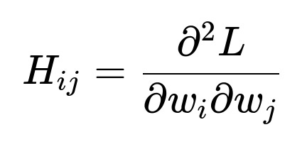
In principle, if H were easy to invert and the problem were convex, Newton’s method converges very quickly to a minimum. But for deep networks, H is huge, non-sparse, often ill-conditioned, and costly to compute. The need to invert such a large matrix, or even approximate it at each iteration, is not feasible at large scale.

Memory and Computational Complexity Analysis

Computing and storing the Hessian has a memory complexity on the order of the number of parameters squared. Inverting or factorizing such a matrix would generally be on the order of the cube of the number of parameters in the worst case, which is never practical for neural networks with millions to billions of weights.

In contrast, computing gradients is linear in the number of parameters (given a single batch). The repeated gradient evaluations in first-order methods remain tractable, which is one reason these approaches remain the de facto standard in deep learning.

Where Newton-Like Methods Could Be Useful

In lower-dimensional problems, second-order methods can indeed converge much faster. For small networks or certain convex optimization tasks (e.g., classical machine learning algorithms with relatively few parameters), approximate second-order approaches or quasi-Newton methods can be beneficial. These are rarely used at scale for training deep networks due to the reasons outlined, but in specialized scenarios or for hyperparameter optimization in lower-dimensional spaces, second-order techniques can sometimes be viable.

Potential Follow-up Questions

Why is the Hessian often ill-conditioned in deep learning, and how does this complicate second-order optimization?

In typical high-dimensional loss landscapes of deep neural networks, you might have plateaus, saddle points, and other non-convex features that lead to eigenvalues of the Hessian spanning a wide range, including negative and very small positive values. This makes the matrix ill-conditioned, so small errors in Hessian estimation can be amplified significantly, and inverting or factorizing such a matrix leads to numerical instability. In practice, this means that even if you could compute the Hessian, its inversion might steer the parameter updates in the wrong direction if the estimation or conditioning is poor.

There are also phenomena like saddle points with many small positive and negative curvature directions that appear in deep learning. Newton’s method may need advanced modifications, such as damping or regularization, to avoid amplifying these negative directions, but that further complicates the approach and reduces its purported rapid convergence advantage.

How do quasi-Newton methods such as L-BFGS help mitigate the full Hessian computation, and why are they still not the norm?

Methods such as L-BFGS attempt to approximate the Hessian or its inverse using limited memory representations. Instead of forming the full Hessian, they rely on gradient differences across iterations to build an approximation to the curvature. This lowers memory usage somewhat because they only store a few vectors related to recent gradient updates.

However, even these reduced-memory approximations can become expensive in large neural networks. They still have greater overhead than simpler first-order methods. Additionally, there is no guarantee that the approximate Hessian remains well-conditioned or captures the true curvature in highly non-convex, high-dimensional loss surfaces. Consequently, simpler first-order methods often yield faster results in practice, especially if you exploit large-scale parallelization or mini-batch optimization.

Are there scenarios where second-order methods might be beneficial in deep learning?

They can be beneficial in tasks like fine-tuning or training smaller models, or perhaps when dealing with specific sub-modules that have a smaller parameter space. Another area is in meta-learning or hyperparameter tuning, where certain second-order information can help optimize hyperparameters or adapt more efficiently. Even in these cases, second-order methods are typically approximate, focusing on partial Hessian information (e.g., diagonal approximations) rather than the full matrix.

There have also been research attempts on methods like K-FAC (Kronecker-Factored Approximate Curvature), which approximates blocks of the Hessian using Kronecker products. These reduce some computational burdens and can leverage matrix factorization tricks, but they are still more expensive than straightforward gradient descent and remain an active research area rather than a universally adopted tool.

What practical trade-offs come into play if one tries to implement a second-order method for a large neural network?

The major limitations revolve around the overhead in time and memory. Constructing Hessian approximations, storing intermediate factorization results, and the added numerical instability from inverting large matrices can outstrip the raw advantage of fast convergence per iteration. When training large models, you usually rely on distributed computing frameworks that parallelize gradient computation across many devices. A second-order approach would demand even more intensive communication overhead, especially if one tried to gather full or partial Hessian approximations across workers. This can slow down the overall training pipeline compared to a simpler first-order approach that just aggregates gradients.

Another trade-off is complexity of implementation and tuning. Stochastic gradient-based methods (like SGD or Adam) have well-understood hyperparameters and are straightforward to implement. Second-order methods need more advanced, carefully engineered heuristics (e.g., damping, line search strategies, approximate inverses) to remain stable, which introduces more potential failure modes in practical training scenarios.

How do modern optimization practices in deep learning address curvature without using the full Hessian?

Adaptive first-order optimizers like Adam, RMSProp, and Adagrad keep track of per-parameter or per-dimension variance estimates of the gradient. By scaling each parameter’s update according to local gradient variance, these methods approximate the idea of normalizing updates by local curvature, albeit in a heuristic manner.

While these do not incorporate the full second-order information like the Hessian cross-covariances, they often provide enough adaptivity to speed up convergence in practice. They also remain relatively cheap, requiring only simple moving averages of squared gradients instead of a full matrix. This is typically why many practitioners find them effective for a wide range of deep learning tasks.

How do saddle points differ from local minima and why can they be problematic for Newton’s method?

A saddle point is a location in the parameter space where the gradient is zero but where the Hessian has both positive and negative eigenvalues. This means the loss function curves upward in some directions and downward in others. For high-dimensional functions typical in deep learning, saddle points are believed to be more prevalent than local minima. One reason is that the measure of strict local minima in such spaces can be relatively small, and the parameter space can contain many high-dimensional saddle points.

Newton’s method near a saddle point can behave unpredictably because the Hessian is indefinite and inverting it without proper regularization might move the parameters toward a direction of increasing loss. Gradient descent methods, on the other hand, have simpler update rules that do not rely on inverting the Hessian and are typically less sensitive to these pathological curvature directions.

Why do we say Newton’s method has quadratic convergence, and does that apply to non-convex problems like deep learning?

In a purely convex setting where the Hessian is positive definite, Newton’s method can exhibit quadratic convergence near the optimum. This means that once the solution is close enough, the distance to the optimum can decrease roughly by the square of the previous distance in each iteration. This property is a powerful theoretical advantage when dealing with well-behaved problems such as logistic regression with relatively few parameters.

In deep learning, the loss surfaces are non-convex, have many local minima, saddle points, and other complexities. The Hessian may not be positive definite, and the function may not behave in the smooth manner required for guaranteed quadratic convergence. As a result, the theoretical fast convergence arguments do not cleanly carry over, so Newton’s method loses much of its attractiveness.

Could second-order methods be combined with methods for gradient estimation to reduce their cost?

Researchers have explored techniques that sample subsets of parameters or data to build a stochastic approximation of the Hessian. Examples include subsampled Hessian approaches or diagonal/low-rank approximations. While these reduce the cost, they still require more overhead than simple gradient-based updates and can introduce significant estimation noise. Consequently, the best balance between complexity, memory, and convergence rate typically remains in the realm of advanced first-order methods, at least for large-scale tasks.

Are there any real-world examples where a full Newton’s method has been successfully applied to large-scale neural networks?

It is not common to see a full Newton’s method in large-scale scenarios. Most attempts in second-order optimization for deep learning are approximate or quasi-Newton methods (e.g., L-BFGS, K-FAC, Shampoo). These sometimes show promising results in certain specialized tasks, especially smaller networks or single-machine tasks where memory constraints are less severe. But the moment you scale to massive models trained across multiple GPUs or TPUs, the overhead of computing second-order information tends to overshadow any gains from fewer optimization steps. Hence, for real-world production-scale neural network training in FANG companies, standard first-order methods remain the typical approach.

---

Below are additional follow-up questions

How do second-order methods behave when the data distribution shifts during training?

When data distribution changes over time (for example, in non-stationary environments or in continuous learning scenarios), second-order methods can become especially problematic. With gradient descent or its variants, you adapt quickly by simply adjusting the step size and continuing to compute gradients on the new data. The overhead is relatively small because first-order methods only need the immediate gradient of the new samples.

For second-order methods, you not only need updated gradient information but also an updated Hessian approximation. If the data distribution shifts significantly, the previously estimated Hessian (or approximate Hessian) may no longer reflect the correct curvature on the new data. Re-estimating or even incrementally updating the Hessian can be computationally expensive and subject to large errors when the distribution shift is large.

In edge cases where distribution shifts are slight, a second-order method might still be feasible if you use a low-rank approximation of the Hessian or a running estimate (like certain quasi-Newton approaches). However, as soon as the shift becomes more pronounced, the mismatch between the old curvature estimate and the new reality can lead to improper updates and possible divergence in training.

What about second-order methods for very large language models (LLMs) where the training set is extremely diverse?

When training large language models with billions of parameters across enormous datasets (spanning diverse domains and languages), the Hessian becomes even more unwieldy because of both the size of the parameter space and the heterogeneity of the data. Each mini-batch may represent a tiny fraction of the overall data distribution. Even if you could compute a Hessian on that mini-batch, it might be a poor representation of global curvature.

Moreover, large language models are usually trained in distributed frameworks that split the model across multiple machines or use a data-parallel strategy. Gathering and synthesizing Hessian information across many nodes is expensive in terms of communication overhead. The reduction (all-reduce or similar operations) needed for first-order gradients is already non-trivial. Extending that to second-order computations, which would require additional sets of partial derivatives or Hessian-vector products, can severely degrade throughput.

In rare specialized scenarios, researchers may try approximate second-order techniques for specific phases of training (e.g., in fine-tuning or for certain layers), but a full second-order approach remains intractable for typical large-scale language model training. This is an acute pitfall in real-world production settings where the cost in memory, compute time, and distributed synchronization makes second-order methods nearly impossible to deploy at scale.

How do second-order methods compare when dealing with extremely sparse gradients or highly regularized settings?

In highly regularized settings, such as when strong or regularization is applied, the shape of the loss function can become more tractable in some directions but remain complex in others. Sparse gradients often occur in models with embeddings or certain activation patterns. For first-order methods, sparse updates can be beneficial because you only update a subset of parameters for each mini-batch.

With second-order methods, you must consider the curvature of the entire parameter space. If many gradients are zero or near-zero, a naive second-order approach may incorrectly interpret large Hessian diagonal entries (or off-diagonal interactions) in certain directions. This can lead to large or erratic parameter updates in directions that are effectively “frozen” or meant to remain sparse.

A subtle pitfall arises when the Hessian includes many near-zero entries corresponding to these sparse dimensions. Approximations to the Hessian may incorrectly amplify noise, especially if the matrix is ill-conditioned. Handling regularization terms with second-order methods can also complicate the Hessian calculation, since you have to incorporate second derivatives of the regularization term (which, in the case of , is not differentiable at zero). Specialized handling for is required, making second-order approaches significantly more complex in implementation.

Could second-order information lead to faster escape from certain saddle points, or does it sometimes hamper it?

There is an argument that second-order information can help detect negative curvature directions and potentially escape saddle points more quickly. In particular, if the Hessian has negative eigenvalues, a second-order method can, in principle, exploit that curvature to move in directions that reduce the loss, bypassing the flat directions where the gradient might be very small.

In practice, the theoretical advantage can be overshadowed by numerical instability. Accurately identifying those negative curvature directions may require carefully factoring or approximating the Hessian to capture negative eigenvalues. Moreover, in a high-dimensional space, saddle points can be extremely flat in many directions, and limited-memory Hessian approximations might miss those subtle negative curvature directions altogether.

A potential pitfall is that if you approximate the Hessian poorly, you might amplify noise or push parameters in a detrimental direction. Empirically, simpler techniques such as a momentum-based gradient approach can often escape from saddle regions without the overhead of computing second derivatives.

Does the curvature estimated by second-order methods become outdated quickly during rapid training phases?

During early training, the parameters of a deep network can shift significantly after each mini-batch update. If you are attempting to use a second-order method, any Hessian or inverse Hessian approximation you compute at one iteration may become outdated within a few steps, especially if the learning rate is relatively large or if the network undergoes rapid structural changes (such as changes in activation patterns).

This is a serious drawback because the potential benefit of second-order methods hinges on reusing curvature information across multiple steps, expecting that the local curvature doesn’t change drastically. If the curvature changes quickly, your expensive Hessian approximation becomes obsolete just as fast, negating any convergence advantage. Consequently, you might spend more computational resources than necessary on updating second-order statistics that do not provide long-term benefits.

How might second-order optimizers deal with batch normalization or other layers that introduce additional non-linearities?

Batch normalization layers, dropout, and other stochastic or stateful components can complicate the curvature landscape. For instance, batch normalization changes the distribution of activations based on the statistics (mean and variance) within a mini-batch. These changing distributions in turn alter the effective loss surface, which can differ from iteration to iteration.

For second-order methods, it’s already challenging to compute or approximate the Hessian in a stable manner. Introducing batch normalization means that the relationship between parameters and outputs is more dynamic, depending on mini-batch statistics. In a first-order method, you simply compute the gradient each time, and it inherently accounts for how the forward pass changed. But for second-order methods, tracking how the Hessian evolves under batch normalization is significantly more complex.

One might attempt to freeze batch norm parameters (or use fixed running statistics) while estimating Hessian information, but that introduces an artificial discrepancy between the real training dynamics and the Hessian approximation. This mismatch can lead to suboptimal or incorrect second-order updates, especially in large networks that rely heavily on batch normalization.

What are the considerations for second-order methods in reinforcement learning (RL) contexts?

In reinforcement learning, gradient updates typically come from stochastic estimates of long-term returns rather than direct supervised targets. The variance in these gradient estimates can be high, especially if reward signals are sparse or delayed. A second-order method in RL would attempt to incorporate curvature information from these noisy gradient signals, but the noise can make Hessian estimation extremely unreliable.

Furthermore, in many RL environments, data distribution is non-stationary because the policy changes over time, leading to new states and transitions. As in non-stationary supervised learning, the Hessian would need frequent updates, each of which is costly. Another subtle pitfall is that partial observability or exploration strategies can drastically alter the trajectory distribution, making it even harder to maintain a stable second-order approximation. As a result, first-order methods like policy gradient or actor-critic approaches remain more prevalent in RL.

How do second-order approaches handle enormous parameter tying, such as in shared embedding matrices or weight sharing across different modules?

Many large neural architectures reuse parameters. For instance, language models often share embedding matrices between inputs and outputs, or convolutional neural networks may reuse weights in repeated blocks. Weight sharing reduces the effective number of free parameters, but from a second-order perspective, the curvature can still be large and complicated because each shared parameter affects multiple parts of the network differently.

When a single weight is reused in multiple modules, the Hessian sub-block that corresponds to that parameter can have complex off-diagonal interactions. It’s not just a simple diagonal or local block structure. A naive second-order method might fail to capture these subtle correlations unless it explicitly models the block structure introduced by weight sharing.

Pitfalls arise when approximate Hessian methods assume independence between parameters that are actually heavily coupled. You might get incorrect curvature estimates that hamper stable convergence. Fine-tuning these approximations can require specialized knowledge of how the network shares parameters, further complicating the implementation and diminishing the advantage of a standard second-order routine.

Are there scenarios where second-order methods might cause slower convergence if the Hessian approximations are inaccurate?

Yes, if the Hessian approximations are poor or out of date, the update direction can be worse than a simple negative gradient direction. In an extreme case, a badly conditioned Hessian inverse approximation can produce a parameter update that substantially increases the loss. This forces you to either reduce the step size drastically or revert to safer methods, negating the benefit of second-order curvature knowledge.

In a typical training loop, you might try a line search to ensure the update step doesn’t overshoot. But this adds overhead (evaluating the loss function at multiple points) and is still vulnerable if the Hessian approximation is systematically biased in certain directions. For large networks, frequent inaccurate approximations are more likely due to higher variance in gradient signals and non-convexities, leading to scenarios where second-order steps fail to converge faster and can even oscillate or diverge.

How do second-order methods handle gradient clipping, which is commonly used in training large networks?

Gradient clipping is used in many large-scale training runs to avoid exploding gradients, especially in recurrent networks or certain transformer architectures. If you try to apply second-order techniques, you have to decide how to incorporate clipping. A naive approach might compute the Hessian first, but once you perform gradient clipping, the direction and magnitude of your gradient (and hence the approximate curvature) changes.

You could attempt to incorporate the clipping operation into the Hessian computation, but that becomes a piecewise operation. Once clipping occurs, the gradient is no longer a smooth function of the parameters, further complicating the second derivative calculation. If clipping is triggered often, large portions of the Hessian might be incorrect. This mismatch can lead to unstable or meaningless second-order updates. In practice, most second-order methods are not designed to handle frequent clipping gracefully, another reason they’re rarely used in real-world scenarios where gradient clipping is standard practice.

Can second-order methods be stabilized by combining them with robust loss functions or gradient smoothing?

One idea is to use robust loss functions that reduce the influence of outliers, or to apply gradient smoothing techniques so that the gradient remains stable between updates. This might help second-order methods by preventing extreme Hessian values from overshadowing the average curvature. However, even then, second-order updates may remain vulnerable if the fundamental shape of the loss surface is still highly non-convex or if the dimension is very large.

Robust loss functions don’t necessarily simplify the Hessian structure; they only bound the influence of large errors in the gradient. The Hessian can still be large, noisy, and difficult to invert. Gradient smoothing might limit the volatility, but it also introduces a bias in the gradient estimates, potentially causing suboptimal or slower convergence if you rely on the exact curvature. There is a trade-off between making the data distribution “nicer” for curvature estimation and introducing distortions that hamper the fidelity of the gradient. This compromise rarely results in a clear advantage over simpler first-order adaptivity.

How might second-order methods be integrated with modern large-scale distributed frameworks without overwhelming network bandwidth?

In distributed training, data-parallel or model-parallel approaches typically only need to exchange gradients or partial gradients among workers. A second-order approach would need significantly more data transfer to communicate Hessian information or approximate Hessian statistics. This can saturate network bandwidth or demand specialized hardware interconnects.

Some research prototypes compress or quantize the curvature information to reduce communication volume. However, compression can induce errors that further degrade the quality of the Hessian estimate. Moreover, these advanced frameworks are complex to implement and maintain. Even if you reduce the communication cost somewhat, the overhead of gathering and inverting (or factorizing) the approximate Hessian remains formidable. Therefore, it is still a niche area compared to the routine practice of exchanging first-order gradients.

Are there specialized hardware accelerators that could make second-order training more feasible?

In principle, if specialized hardware existed for fast matrix operations or matrix inversions at the scale of neural network Hessians, second-order methods might become more practical. Modern GPUs, TPUs, or custom accelerators excel at matrix multiplications for forward/backward passes, but they are not specifically designed for repeated Hessian computations and large-scale matrix inversions.

Even if you had hardware that made large matrix inversions more tractable, you would still face the fundamental challenges of ill-conditioning and non-convexity. The advantage of second-order methods is most pronounced in well-conditioned, convex problems. For deep networks with complex architectures and huge parameter counts, no hardware can magically resolve these algorithmic and mathematical challenges.

Could second-order methods be useful after an initial phase of training, once the network is close to a local minimum?

One strategy might be to train with a first-order method initially to reach a region near a local or global minimum, then switch to a second-order method to refine the solution. This approach assumes that once you are near a minimum, the Hessian becomes more stable and easier to approximate. If the Hessian is nearly positive definite near that solution, Newton-like steps can converge quickly.

However, even near the final stages of training, the memory cost of second-order information remains prohibitive for large networks. Also, if the local minimum is in a very flat region, the Hessian might still have small or zero eigenvalues, and that can frustrate accurate inversion. There could be an incremental benefit in certain tasks requiring extremely high precision of final solutions, but for many deep learning applications, small differences in the final loss do not necessarily translate to large improvements in generalization. Hence, the incremental payoff of second-order refinement is often not worth the additional computational overhead.