
ML Interview Q Series: Optimizing Tour Boat Schedules with Poisson Arrivals using Renewal Reward Theory.

Browse all the Probability Interview Questions here.
14E-12. A canal touring boat departs for a tour through the canals of Amsterdam every T minutes with T fixed. Potential customers pass the point of departure according to a Poisson process with rate λ. A potential customer who sees that the boat leaves s minutes from now joins the boat with probability e^(-μ s) for 0 ≤ s ≤ T. Assume that a fixed cost of K>0 is incurred for each round trip and that a fixed amount R>0 is earned for each passenger. Identify a regenerative stochastic process to find the long-run average net reward per unit time as a function of T. What value of T maximizes this long-run average net reward? Hint: use the fact the arrival time of the n-th potential customer has the density ( (λ t)^(n-1) e^(-λ t) ) / (n-1)!, and use conditioning to find the probability that the n-th arrival joins the first trip of the touring boat.
Short Compact solution
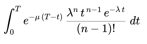
By conditioning on the arrival time of the n-th potential customer and using the law of total probability, the probability that this n-th arrival joins the first trip is:
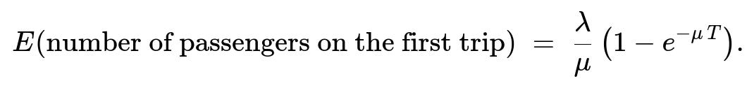
Summing over n from 1 to ∞ and interchanging the order of summation and integration (while using the identity ∑ (λ^n t^(n-1) e^(-λ t)) / (n-1)! from n=1 to ∞ = λ), one obtains the expected number of passengers on the first trip:
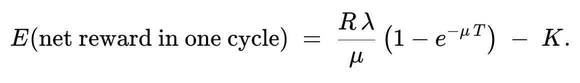
Hence, the expected net reward in one cycle (the time between consecutive departures, which has length T) is
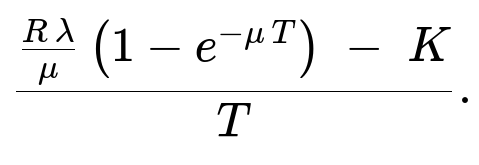
By the renewal-reward theorem, the long-run average net reward per unit time is
Assuming Rλ/μ > K, we differentiate with respect to T, set it to zero, and solve for T to find the unique maximizing solution. The resulting condition can be written as:
That T is the unique value that maximizes the long-run average net reward per unit time.
Comprehensive Explanation
Identifying the Regenerative Process A process {X(t), t ≥ 0} is said to be regenerative if there are random times, called regeneration epochs, at which the process probabilistically “restarts” itself. In this problem, the departure epochs of the boat act as natural regeneration points. After each boat departure, the system “resets” in that you begin waiting for the next T-minute interval until the next departure. From that point onward, the arrival and joining behavior of customers is the same as in all previous cycles.
The Expected Number of Passengers per Cycle Within each T-minute cycle, potential passengers arrive according to a Poisson process with rate λ. If there are n arrivals in the interval [0, T], the n-th one occurs at a time that follows the Gamma(n, λ) distribution (or equivalently an Erlang distribution). Condition on the event that the n-th arrival time is t. The probability that this n-th arrival decides to join the boat, given that the boat leaves at time T and the current time is t, is e^(-μ (T - t)), where 0 ≤ t ≤ T.
Summing this joining probability over all possible arrival counts n, and integrating over the arrival time t from 0 to T, yields the expected number of passengers boarding the boat in that cycle. Interchanging the summation (over n) and the integral (over t), and using the fact that for each fixed t,
∑ from n=1 to ∞ of [ λ^n t^(n-1) e^(-λ t ) / (n-1)! ] = λ
completes the derivation that the expected number of passengers per cycle (i.e., per T-minute period) is ( λ / μ ) (1 - e^(-μ T)).
Expected Net Reward per Cycle Each passenger contributes a fixed reward R, so with an expected ( λ / μ ) (1 - e^(-μ T)) passengers per cycle, the expected revenue in one cycle is R times that quantity. We also have a fixed cost K for operating the boat once every T minutes (one cycle). Hence the expected net reward in one cycle is:
( R λ / μ ) (1 - e^(-μ T)) - K.
Using the Renewal-Reward Theorem Each T-minute interval is a renewal cycle. The renewal-reward theorem states that for a regenerative process, the long-run average reward per unit time is the ratio of the expected reward in one cycle to the expected length of one cycle. Since the expected length of each cycle is T, the long-run average net reward per unit time becomes:
( [ R λ / μ ] (1 - e^(-μ T)) - K ) / T.
Maximizing the Long-Run Average Reward We want to find the T that maximizes the expression above. To do this in practice, one typically takes the derivative with respect to T, sets it to zero, and solves for T. Under the assumption that Rλ / μ > K (which ensures a positive solution), one arrives at the condition:
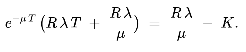
e^(-μ T) ( R λ T + (R λ / μ ) ) = ( R λ / μ ) - K.
The solution T to this equation gives the unique optimum. If Rλ / μ ≤ K, the cost is too high relative to the revenue rate, so the optimal T might degenerate to an extreme (for instance, not operating at all or something similar).
Potential Follow-Up Questions
1) Why does each departure epoch act as a regeneration point?
Between departures, the number of arrivals and their decisions are governed by the same Poisson process and the same joining probability as any other cycle. Once the boat departs, the process “resets” to having zero people waiting and a fresh T-minute period until the next departure. This independence from cycle to cycle is precisely what defines regenerative behavior.
2) What if T is extremely small or extremely large?
If T → 0, the boat departs too frequently. Although you might minimize the waiting time that discourages customers, you likely don’t pick up many because they do not have enough time to arrive. This can result in mostly empty trips and high operating costs per passenger.
If T → ∞, you allow many arrivals to accumulate, but they might choose not to join because s (their wait time) becomes large and e^(-μ s) could become very small. Also, you operate fewer trips, so if the waiting probability decays rapidly, you might lose potential passengers.
3) How do we solve the equation e^(-μ T) (Rλ T + Rλ/μ) = Rλ/μ - K in practice?
You typically do so numerically because this transcendental equation may not have a simple closed-form solution. One might use a numerical root-finding method such as Newton-Raphson or a bisection method. In practice, you guess an initial T, iterate the equation or use derivatives, and converge to the unique positive root.
4) What if there is a maximum capacity on the boat?
The current model assumes an unlimited capacity. If there is a capacity limit, the analysis becomes more complicated because not all arrivals can board if the boat is full. One might then need to account for the probability that the boat is at capacity. The renewal arguments can still apply, but the expression for expected passengers per trip would be capped by the capacity.
5) Could the process still be regenerative if costs or rewards changed dynamically?
Yes, as long as the process “resets” itself at each boat departure in a way that future evolution is independent of the past, except for the state at the beginning of the cycle. However, if costs or rewards are not fixed per cycle or if the system’s state at departure depends on more complicated historical factors, additional considerations or more general forms of renewal processes might be needed.
6) What are practical considerations for choosing μ?
The rate μ captures how quickly people lose interest if the wait is longer. In a real system, μ might reflect average patience or might be empirically estimated. Accurately knowing μ is crucial to ensuring the theoretical maximum is relevant in practice. Real data might show that people’s patience is not strictly exponential; in that case, exponential is an approximation.
7) How would you handle uncertainty in R or K?
In many real applications, the per-passenger reward R might vary (e.g., if there are discounts at off-peak hours), and the cost K might have both fixed and variable components (e.g., fuel costs that scale with the number of passengers). You could modify the model accordingly, but the renewal approach remains valid as long as each cycle is identical in structure and resets at departure.
8) Could a time-varying arrival rate be handled?
If λ changed over time (for example, more tourists arrive at peak hours and fewer at night), then the process in a single cycle wouldn’t have the same distribution if repeated throughout the day. One might either segment the day into periods with approximately constant λ or use a more sophisticated nonstationary Poisson process model. However, the simple renewal method here applies directly only if each cycle is identically distributed.
Below are additional follow-up questions
1) How does the assumption of exponential joining probability (e^(-μ s)) influence the model’s realism?
Answer
In the problem, each potential passenger decides to join with probability e^(-μ s), where s is the time until the boat departs. This choice captures a memoryless “patience” with respect to wait time: the longer the wait, the more likely the person is to become disinterested. However, in the real world, people’s patience may not strictly follow an exponential decay. Some individuals might tolerate a certain threshold wait time without any drop in probability, then sharply lose interest afterwards; others might become only slightly less likely to join over time rather than following a strict exponential curve.
If the true patience distribution differs significantly, then the derived formula for expected passengers (and hence expected net reward) might not hold exactly. One pitfall is that fitting an exponential to data where the hazard rate changes with time (e.g., people might become more impatient as they realize the wait has become lengthy) can lead to systematic errors. Despite this, the exponential form can be a good first approximation when arrivals and decisions are random and memoryless.
In practice, you might gather data on how passengers decide to board or walk away depending on posted wait times and attempt to estimate a more general waiting-time sensitivity function. Nonetheless, if you maintain the renewal structure, you can still form a cycle-based analysis; you just need the correct functional form of the joining probability in place of e^(-μ s).
2) What happens if there is a queue of potential passengers who have partially committed before T is reached?
Answer
The current model assumes that each individual either decides to join or not at the moment they arrive. There is no partial-commitment or reservation concept before the departure time. However, in reality, some systems allow passengers to purchase tickets ahead of departure (for instance, an online purchase or a physical queue forming).
If such partial commitment is possible, you could end up with a queue where people who arrived earlier already “reserved” a seat. This changes the probability of new arrivals deciding to join if they see a partially full or fully booked boat. It could also mean the decision is not merely about the waiting time s but about s plus the uncertainty of seat availability. The Poisson arrivals might still hold, but the joining probability depends on both the wait time and the queue state.
One might then need a more detailed state descriptor: how many seats are “reserved,” how many arrivals have come, and how far the system is from departure time T. The regenerative property can still exist if the state resets after every departure, but the calculation of expected passengers is more complicated. You’d handle it via a continuous-time Markov chain or by conditioning on both the arrival times and the evolving queue length.
3) Could we incorporate group arrivals or batch arrivals instead of individual arrivals?
Answer
The current model relies on a standard Poisson process assumption: arrivals happen one at a time, independently of each other. However, if tourists often arrive in groups (e.g., families), or if there are busloads arriving at once, the arrival process would more accurately be modeled as a batch Poisson process or some other correlated arrival process.
In such cases, the single-parameter Poisson rate λ may not capture the distribution of group sizes. Instead, you would have:
A process for the arrival of the groups (still possibly Poisson),
A distribution for the size of each group (which could be geometric, Poisson, fixed, etc.),
A decision probability for each group or each individual within the group based on remaining time until departure.
This complicates the expected passenger calculation, because the arrival of a large group can significantly alter the average boarding counts. One might still apply a renewal argument each time the boat departs, but the summation to find the expected number of joining passengers would need to account for group size distribution. A common pitfall is to continue to assume a simple Poisson process for individuals when real traffic is more bursty and correlated, leading to underestimates or overestimates of passenger loads.
4) What if boat departure can be delayed or accelerated depending on how many people have shown up?
Answer
In this problem, we fix the departure interval T. However, an operator might consider dynamically adjusting departure times: if many people are waiting, leave earlier; if few are waiting, wait a bit longer to gather more. This no longer maintains a strict T-minute cycle and can break the simple regenerative structure. The system might still be regenerative if it resets upon departure, but each cycle length is now a random variable, not a constant T.
The advantage could be higher average occupancy, but the modeling becomes more intricate. One would have to calculate the expected time until a certain occupancy or until a threshold is reached, and how arrivals keep coming in that window. The cost function might also shift if waiting longer costs you more. This more adaptive policy may yield a higher net reward, but you lose the simplicity of a fixed T and the direct formulas we have. You might need to solve a dynamic optimization or Markov decision process.
A major pitfall is that indefinite waiting could annoy potential passengers if they sense no fixed schedule, reducing future arrivals’ joining probability or damaging the service’s reputation.
5) How does the model change if there is a minimum passenger requirement to justify a trip?
Answer
In many tour operations, there might be a minimum number of passengers needed (let’s call this minimum M) for the operator to deem a trip worthwhile. If the expected number of passengers by time T is below M, the operator might decide to wait longer or even cancel the trip. This creates a random departure time or a cancellation event. As a result, T is no longer fixed but is conditional on whether you reach that minimum number M first.
Mathematically, you must track how many arrivals have decided to join and at what times. If you reach M joined passengers before T, you might depart immediately (or at least consider it). If you do not reach M by T, maybe you cancel or run anyway at a loss. This is no longer a pure renewal with a fixed cycle length because departure times become random. The process can remain regenerative if you define the new cycle as “from the time you start trying to form a trip until the time you either depart or cancel.” You then need to compute the expected cycle length and the expected reward carefully under these more complex conditions.
6) Could the system benefit from offering discounts as departure time approaches?
Answer
In practice, an operator might increase the joining probability by offering lower fares as T - t gets large. That is, if departure is soon, a cheaper fare might encourage people to join quickly. This modifies the revenue per passenger (R becomes R(t)), and also changes the probability function. The question is whether the net effect (increased boarding probability times a possibly lower fare) raises or reduces overall profit.
The renewal setup can still hold, but we have a function R(t) for the revenue per passenger if they arrive at time t, and a probability p(t) of joining that might be higher than e^(-μ (T - t)) if discounted. You must integrate across the interval to find the total expected revenue, then subtract cost K, and then divide by T to find the long-run rate. A subtle pitfall is that if you offer too deep a discount, the average passenger revenue might drop below the threshold needed to cover costs, negating the benefit of having more passengers.
7) Are there any implications if the Poisson arrival rate λ changes mid-cycle due to external events?
Answer
Even if λ is constant on average, real situations can produce spikes (e.g., a large tour bus arrival at time t=5 minutes) or dips (lunch break, off-season) within a single T-cycle. If λ is truly nonstationary within the cycle, you would need a function λ(t) that describes how arrivals vary in time. For instance, if λ(t) is higher in the first half of the cycle than the second, then the distribution of arrival times is no longer uniform on [0, T] with a single rate.
The main pitfall is that the simple step of factoring out λ from the integral and summation no longer holds. You would need to keep track of the time-dependent arrival process in your integration. Although the process might remain regenerative (each departure still resets the clock), the expected count of arrivals who join in each cycle can differ significantly from the expression (λ/μ)(1 - e^(-μ T)). You would do a more general integral with λ(t) inside. This can drastically change the formula for the optimal T.
8) How could one account for passenger heterogeneity in willingness to wait?
Answer
In the model, all arrivals have the same parameter μ, meaning they share an identical exponential waiting tolerance distribution. In reality, some passengers may be extremely patient, while others may be very impatient. A more realistic approach might assign a random patience factor μ_i for each new arrival or, equivalently, a distribution of waiting times to “impatience.”
When you sum up the probabilities of joining, you would now have a mixture of exponentials or an entirely different waiting-time tolerance distribution. That mixture complicates the integral for E(number of passengers), because it becomes an integral over t for the arrival time, multiplied by an expectation over the distribution of μ_i. One might write:
Expected number of passengers = ∫ from 0 to T of [ Poisson-arrival density * E( join probability | arrival at t ) ] dt,
where E(join probability | arrival at t) is an average over different μ_i types. If you keep T fixed, you still have a renewal structure, but the algebra to obtain a closed-form expression might be significantly more involved. Pitfalls arise if you average all passengers into a single μ, since you could underestimate or overestimate actual boardings depending on how skewed the distribution of patience is.
9) In practice, how would you validate or test the theoretical optimum T found from the model?
Answer
After solving for T mathematically, you must ensure that the assumptions align with real operational data. One standard approach is:
Collect real arrival data: Observe arrivals over multiple days and estimate λ.
Observe join behaviors: Record how many potential customers wait and board at varying time-to-departure intervals; estimate an effective μ or measure an empirical distribution of waiting tolerance.
Test different T values: In an A/B testing fashion, operate the boat with different scheduled intervals T. Measure actual revenue and cost over a suitable period, ensuring you gather enough samples for statistical significance.
Compare results to the theoretical prediction: See if the measured net reward per unit time aligns with ( [R λ / μ] (1 - e^(-μ T)) - K ) / T. Any divergence might indicate that λ or μ is misestimated or that real behaviors deviate from the exponential model.
A subtle but common pitfall is ignoring external factors that disrupt your schedules, such as weather, promotional events, or changes in tourism patterns. Even once you pick an optimal T from the formula, unexpected real-world fluctuations might require revisiting the parameter estimates to ensure the model still holds.