ML Interview Q Series: Optimizing with Regularization: Achieving Sparsity via Subgradient Handling.

📚 Browse the full ML Interview series here.

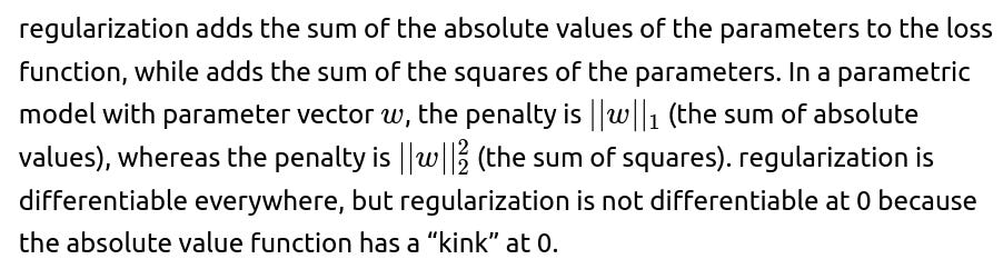
vs Regularization (Optimization Perspective): Contrast and regularization in terms of how they impact the optimization of model parameters. Why does regularization tend to produce sparse solutions (many parameters exactly 0), and how is the subgradient at 0 handled for during optimization?

Below is a thorough exploration of the question, followed by several potential follow-up questions (in H2 format) with in-depth answers.

Why Regularization Produces Sparse Solutions and How the Subgradient Is Handled at 0

Conceptual Overview of vs

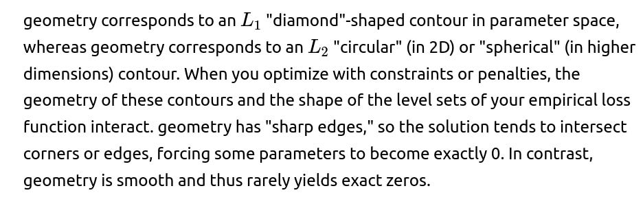
Geometric Interpretation

Optimization Perspective

Sparsity from

Because of the way subgradients behave at 0, regularization can “shrink” parameters to 0 in a discrete jump. Once a parameter hits 0 (because the learning step overcame the threshold), the subgradient can keep it there if that is optimal. This phenomenon is responsible for the sparsity we see in solutions.

Handling the Subgradient at 0

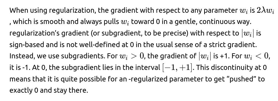
At 0, the gradient of ∣w∣ does not exist in the classical sense. Instead, the subgradient set at 0 for the absolute value term is the interval [−λ,+λ] (if λ is the regularization coefficient in front of the term in the loss). Optimizers that handle typically use proximal gradient methods or some specialized approach that handles this subgradient. In practice, frameworks like TensorFlow or PyTorch may implement penalties by computing sign-based updates combined with special-case handling for those parameters whose absolute values are close to or exactly 0.

Why Does Regularization Tend to Produce Sparse Solutions Compared to ?

How Is the Subgradient at 0 Handled for During Optimization?

At 0, the subgradient lies in the interval [−λ,+λ]. Many practical optimizers implement a “soft thresholding” step or a proximal update when applying . In a basic gradient-based framework, a proximal step for often looks like:

# Simplified "soft-thresholding" style step
# Not a direct library code, just a conceptual illustration

def update_parameter_l1(param, grad, learning_rate, lambda_):
    # gradient-based update ignoring the  penalty
    new_param = param - learning_rate * grad

    # apply a "soft thresholding" for 
    # basically shrink new_param toward zero by lambda_ * learning_rate
    if new_param > 0:
        new_param = max(0, new_param - learning_rate * lambda_)
    else:
        new_param = min(0, new_param + learning_rate * lambda_)

    return new_param

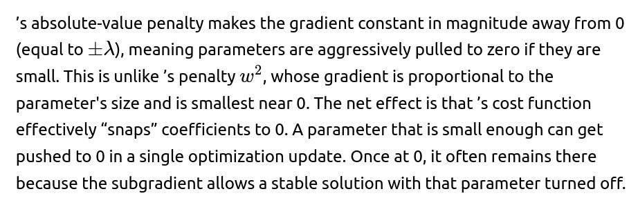
When param is small in magnitude, this update can drive it toward exactly 0. Once param is at 0, it will remain there if continuing to push it toward 0 is beneficial for the objective. This thresholding procedure is the essential reason behind the induced sparsity from .

Possible Follow-up Questions

How does the geometry of and regularization influence the likelihood of sparse solutions?

The geometry of penalty regions has sharp corners (in 2D, a diamond shape), which results in the optimizer hitting “vertices” of that diamond, where some coordinates are forced to 0. In contrast, ’s spherical geometry does not contain any axis-aligned corners, so solutions slide continuously in Euclidean space and rarely land exactly on the axes. This difference in shape is a key visual reason for the frequent appearance of zeros in -regularized solutions.

How do frameworks like PyTorch or TensorFlow implement regularization in practice?

Modern deep learning frameworks often fold into the overall computational graph or rely on specialized optimizers that include a proximal operator. When you specify an penalty in PyTorch, for instance, you might add a term like:

# example of manually adding  penalty to your loss
l1_penalty = 0
for param in model.parameters():
    l1_penalty += torch.sum(torch.abs(param))
loss = original_loss + lambda_ * l1_penalty
loss.backward()
optimizer.step()

Behind the scenes, because the absolute value function is not differentiable at 0, the gradient used is actually a subgradient. If you want exact “soft-thresholding” behavior, you would often need a dedicated routine or a specialized optimizer that implements a proximal step. Standard gradient-based optimizers approximate it with sign-based updates.

Why does a small parameter in an -regularized model often jump to zero while a small parameter in an -regularized model does not?

In , the gradient magnitude for a parameter w away from zero is a constant (either +λ or −λ), so even if the parameter w is small, the pull remains as large as for bigger parameters. In , the gradient magnitude is proportional to w, so very small parameters have a very small gradient, and hence the continuous shrinkage is gentler and less likely to push them all the way to zero in one step.

Could a parameter once set to zero ever leave zero in regularization?

Yes, but only if the gradient of the data-fitting part of the loss is large enough to exceed the boundary set by the subgradient at 0. In practice, once parameters are zeroed out, it may require a large data-driven gradient to “reactivate” them. Often, if the model’s design or learning dynamics do not produce such a large gradient, once a parameter hits zero, it will remain zero.

How do we tune the regularization coefficient for vs ?

In practice, hyperparameter tuning is required, typically by cross-validation. For , the regularization coefficient λ directly influences how many parameters go to zero. A higher λ pushes more parameters to zero, possibly harming accuracy if too many informative parameters are discarded. ’s λ controls how strongly weights are shrunk overall without pushing them exactly to zero. The best practice is to use a systematic search or scheduling approach and track validation error.

When would you choose over (or both via Elastic Net)?

Choose when you need feature selection or prefer a compressed, interpretable model that discards less relevant features. Choose when you don’t necessarily need zeros but want overall smoother, smaller weight magnitudes. Elastic Net is a combination of both, which often helps in high-dimensional settings (like text or genomics) where correlated features appear, because pure might arbitrarily select among them while spreads the shrinkage. Elastic Net yields a compromise between shrinkage and sparsity.

Are there any pitfalls with regularization in large-scale deep learning?

One major pitfall is that the gradient-based updates may not produce as strong a sparsity effect as desired unless you use specialized proximal steps. Another challenge is that setting a large coefficient can kill too many parameters, harming representational capacity. Also, adding to very deep networks can introduce instability in training if not tuned carefully. Finally, in extremely large neural networks (like massive language models), you might not rely purely on to provide interpretability or compression. Pruning techniques or structured sparsity might be more suitable.

Does regularization always guarantee better generalization?

Not always. can help with interpretability and can reduce overfitting by zeroing out irrelevant features, but for some tasks, it might underfit if too many weights are set to zero. might sometimes offer superior predictive performance if interpretability or feature selection are not your main goals. The best solution is usually empirical: test both approaches (or a combination) on validation data.

Does or matter more in extremely high-dimensional spaces?

In very high-dimensional feature spaces with a small number of real informative features, is extremely useful because it systematically removes irrelevant features by driving them to zero. may shrink all features but still keep them in the model, potentially complicating interpretation. Therefore, is often favored for sparse or interpretability-driven setups.

Practical Implementation Example

Below is a brief conceptual code snippet illustrating how one might manually implement gradient updates with an penalty in a PyTorch-like setting. This example is purely for demonstration; in practice, you would rely on library-built optimizers or a specialized proximal step.

import torch

# Suppose we have a simple linear model: y = w * x + b
# We'll do a single training step with  penalty manually.

# Sample data
x = torch.randn(10, 1)
y = 3 * x + 0.5  # "true" slope = 3, intercept = 0.5
y += 0.1 * torch.randn(10, 1)  # a bit of noise

# Parameters
w = torch.randn(1, requires_grad=True)
b = torch.randn(1, requires_grad=True)

learning_rate = 0.1
lambda_l1 = 0.01

for epoch in range(100):
    y_pred = w * x + b
    loss_mse = torch.mean((y_pred - y) ** 2)

    # Add  penalty
    l1_penalty = torch.sum(torch.abs(w)) + torch.sum(torch.abs(b))
    loss = loss_mse + lambda_l1 * l1_penalty

    # Backprop
    loss.backward()

    # Manual gradient descent step
    with torch.no_grad():
        # Basic gradient step ignoring 
        w -= learning_rate * w.grad
        b -= learning_rate * b.grad

        # Reset gradients to zero
        w.grad.zero_()
        b.grad.zero_()

        # Now do the "soft threshold" step for w and b
        # We subtract lambda * lr from their magnitude if > 0
        # and clamp at 0
        if w > 0:
            w = torch.max(torch.tensor(0.0), w - learning_rate * lambda_l1)
        else:
            w = torch.min(torch.tensor(0.0), w + learning_rate * lambda_l1)

        if b > 0:
            b = torch.max(torch.tensor(0.0), b - learning_rate * lambda_l1)
        else:
            b = torch.min(torch.tensor(0.0), b + learning_rate * lambda_l1)

In reality, you would typically rely on a built-in optimizer or a specialized proximal operator method. The key difference from a normal SGD update for is the extra thresholding step that enforces sparsity.

---

Below are additional follow-up questions

How do and differ when the input features are highly correlated, and what are the potential pitfalls?

When input features are highly correlated, regularization tends to distribute weight (or importance) across all correlated features, because its penalty scales with the square of the coefficients. In contrast, regularization prefers to “pick” a subset of correlated features and push the rest to zero, essentially performing feature selection. This can be beneficial if you want a sparser model that relies on fewer features, but there are a few potential pitfalls:

• Instability in feature selection: If several features are equally predictive and correlated, may randomly pick one feature over the others. Small changes in the data or training procedure could cause the chosen non-zero feature set to fluctuate, making the model’s selected features less stable across different training runs.

• Loss of complementary signal: In some datasets, multiple correlated features may each contain small but distinct signals. might end up eliminating some of those correlated features, potentially discarding additional bits of information that could have improved generalization.

• Interpretability trade-off: Sparsity enhances interpretability because you have fewer active features. But if the chosen feature subset is not the only “valid” subset, interpretability might be misleading in the sense that other equally good sets of features might also exist.

In practical terms, if you are in a domain where correlated features abound (e.g., text data with synonyms, genomic data with correlated SNPs, etc.), you must be aware that solutions may be unstable or might throw away useful redundancy. Elastic Net (a combination of and ) is often preferred in such scenarios because it exploits both sparsity () and smooth shrinkage ().

In advanced optimizers like Adam or RMSProp, does still produce sparse solutions, or do we need special handling?

Modern optimizers such as Adam, RMSProp, or Adagrad adapt the learning rate for each parameter based on historical gradients. This adaptation can interact with the constant-magnitude subgradient from . Specifically:

• Sparse solutions can still occur: Even with adaptive learning rates, if the effective gradient step for a parameter is large enough to overcome that parameter’s magnitude, it can be driven to exactly zero. Once zero, the subgradient allows it to remain there unless the main (data) gradient is strong enough to “reactivate” it.

• Potential for overshadowing effect: Adam and similar optimizers compute moving averages of gradients and squared gradients. If the scale of these estimates is large for some parameters, the effective step might overshadow the thresholding effect or make it inconsistent across dimensions.

• Special handling (Proximal or Soft Thresholding): True -based “soft thresholding” can be lost if you rely purely on standard gradient updates. Some libraries or implementations provide a “proximal Adam” or “Adam with weight decay but for .” In these cases, an explicit proximal step is added after each gradient-based update. This step subtracts a constant amount from the parameter magnitude and clamps it to zero if that surpasses the absolute value. This ensures proper sparsity even with advanced optimizers.

• Practical tip: If you do not use a special proximal step, you might find that does not produce as much sparsity as you expected. This is sometimes because the adaptivity of learning rates can reduce the effective magnitude of ’s gradient-based shrinkage.

How does regularization interact with batch normalization or layer normalization in deep neural networks?

Batch normalization (BN) and layer normalization both rescale and shift intermediate activations in a way that can affect how parameters are updated. Key points:

• Scaling of parameters: If you have an penalty on the parameters themselves (e.g., the weights of a convolution layer), the internal scaling from batch or layer normalization does not directly remove or alter the penalty on the raw weight. However, the distribution of activations might reduce or amplify the effective gradient needed to drive weights to zero.

• Reduced internal covariance shift: One of BN’s goals is to stabilize the distribution of activations. This can sometimes make training less sensitive to different parameter scalings, so the interplay with might become less pronounced, especially if the BN layers can “normalize out” large or small parameter magnitudes at activation-time.

• Potential for overshadowed effect: Because BN can learn its own shift and scale parameters, the network can sometimes rely more on these BN parameters to adjust feature magnitudes rather than pushing weight parameters to zero. If your goal is explicit weight sparsity, you might still prefer to apply a specialized approach (like a proximal or thresholding-based method).

• Pitfall with post-BN pruning or re-initialization: If your network heavily relies on BN to maintain stable activations, zeroing weights in certain layers might have a dramatic or negligible effect depending on how the BN parameters readjust. You need to monitor performance carefully if you are using for pruning in tandem with BN.

Are there any scenarios in which regularization might actually harm interpretability?

Although is generally believed to promote interpretability by zeroing out irrelevant weights, it can sometimes compromise interpretability in unexpected ways:

• Over-pruning of correlated features: If multiple correlated inputs each partially contribute to an interpretation, might prune away some features that hold complementary signal. The resulting model might appear simpler but could mask the fact that a more nuanced combination of features existed.

• Sparse yet unstable solutions: The exact set of non-zero features can vary across different random seeds, data splits, or minor hyperparameter changes. This variability can reduce trust in the interpretation of which features are truly critical.

• Misleading sense of importance: In certain networks, a weight going to zero might not strictly mean the feature is entirely unused, especially if the architecture includes skip connections or if multiple parallel pathways can carry the same signal. So, the presence of zero weights might not always map cleanly to a single, unique interpretation path.

Thus, while can give a “cleaner” feature set, you should always validate interpretability claims by cross-checking with domain knowledge and verifying the model’s stability under small perturbations.

How do we handle regularization in the presence of parameter constraints, such as positivity-only weights?

Some models or architectures (e.g., certain economic or probabilistic models) enforce non-negative weights:

• Projected gradient approach: After each gradient step (including the penalty), you project the parameters onto the feasible set (e.g., clamp them to at least 0). In tandem with , you may find that some weights sit exactly at 0, consistent with both the objective and the positivity constraint.

• Proximal methods for constrained optimization: A proximal operator can combine with positivity constraints by performing a “soft thresholding” followed by a positivity clamp (i.e., threshold to zero if it goes negative).

• Edge cases: If your data gradient or penalty is strong enough in the negative direction, you might see many weights clamped to zero due to the positivity constraint. This can produce an even sparser solution than an unconstrained scenario. Conversely, if the positivity constraint is crucial for interpretability (e.g., a weight can’t be negative in the real-world domain), you must ensure that your -based approach doesn’t break the feasible set. Checking boundary conditions at each update is critical.

• Pitfall with certain optimizers: Some built-in optimizers might not handle positivity constraints by default. You must explicitly handle constraints at each step or use a specialized constrained optimizer (e.g., PyTorch’s “projection” hooks or advanced libraries).

Does performing gradient clipping in very large models affect the sparsity induced by regularization?

Gradient clipping typically restricts the norm of the gradient to prevent explosive updates, especially in deep networks with long backpropagation chains. Here’s how it can intersect with :

• Clipped subgradient effect: The subgradient is ±1 away from zero (scaled by the regularization coefficient). If gradient clipping is quite strict, this subgradient might get reduced in magnitude, effectively reducing ’s ability to push weights toward zero.

• Less abrupt parameter updates: If your model frequently hits the gradient clipping threshold, the step for each parameter is scaled down. This can hamper ’s “hard push” to zero, leading to less sparsity.

• Potential solutions: One strategy is to separate the penalty from the main gradient flow and apply a proximal update or a thresholding step after gradient clipping. That way, gradient clipping preserves training stability for the main loss while can still impose strong shrinkage. Alternatively, you can carefully tune the clipping norm to avoid drowning out the effect.

• Real-world subtlety: In extremely large models (e.g., large language models), gradient clipping is common, so might be overshadowed. Practitioners often rely on magnitude-based pruning or structured pruning post-training instead of raw regularization.

Can regularization emulate sparsity if we post-process small weights by thresholding them to zero?

Yes, this is an approach some practitioners use:

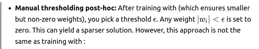
• There is no direct gradient pressure to set weights exactly to zero during training.

• The final set of zeroed weights might not be optimal for the original objective, because the model never saw these exact zeros during training.

• If you re-fine-tune the model after thresholding, you might recover some performance lost by the abrupt removal of weights.

• Comparison to actual : A true approach integrates sparsity into the training objective, so the model “knows” that zero is a candidate solution for certain weights. Post-hoc thresholding with is more of a hack or a two-step pipeline: (1) shrink weights with , (2) prune with an arbitrary threshold, (3) possibly re-train. It can work in practice but does not strictly replicate the dynamics of .

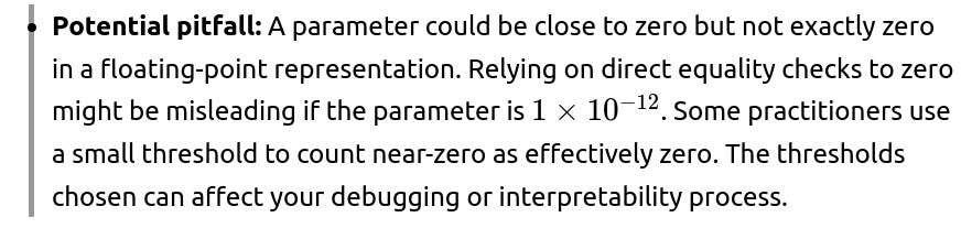
• Pitfall with threshold selection: Choosing ϵ can be non-trivial. Too large and you lose important weights, too small and you gain minimal sparsity. You also must test the performance after thresholding to ensure the model still generalizes well.

Under what circumstances might regularization yield worse performance than using no regularization at all?

Although generally helps control overfitting by enforcing sparsity, there are scenarios where it can backfire:

• Data-limited setting with many correlated features: If you do not have enough data, an overly aggressive penalty might zero out crucial correlated features, resulting in a model that underfits. Without enough data to identify which features truly matter, the penalty might be “guessing in the dark,” causing damage to predictive performance.

• Inappropriate hyperparameter tuning: If the coefficient λ is set too high, the penalty might dominate the data-fidelity term, collapsing nearly all weights to zero. This leaves the model with almost no representational power, significantly hurting performance.

• Feature engineering reliance: In some tasks, each feature by itself might be weak, but many collectively are essential. can be too aggressive, removing a large portion of these subtle features. Without strong domain knowledge to guide usage, the model might fail to capture these weaker signals.

• Non-sparse truth: If the true underlying relationship is not sparse—say most of the features have some partial relevance— might not be the best choice. might be more appropriate, as it shrinks but doesn’t enforce that some features be dropped outright.

• Edge case in deep neural networks: Extremely large networks can adapt to many parameters. Sometimes forcing too few of them to remain active can degrade the benefits of having a wide set of learned representations. This is especially true if your architecture is designed to rely on overparameterization and you are not truly seeking feature elimination.

Could encourage a form of “structured sparsity” in neural networks, or does it only act at the individual parameter level?

Basic regularization typically acts on individual parameters, encouraging each weight to go to zero independently. This is referred to as “unstructured sparsity.” However, many real-world architectures (like CNNs or RNNs) might benefit more from “structured sparsity,” where entire filters, channels, or blocks of parameters are zeroed out together. Standard does not inherently enforce such structure, leading to scattered zeroes. Some considerations:

• Group (Group Lasso): A variation of that penalizes entire groups of parameters with a group norm. For instance, in convolutional networks, you could group all weights of a filter as a single entity. If the group penalty is large enough, the entire filter is dropped. This yields structured sparsity that can speed up inference on specialized hardware.

• Practical advantage of group-based approaches: If you want to reduce memory usage or accelerate computation, unstructured sparsity is sometimes less helpful because random zeroes are harder to exploit on standard hardware. Structured sparsity is more hardware-friendly, as entire filters or neurons can be skipped.

• Implementation detail: Many deep learning frameworks do not provide built-in group , so you might need custom code or specialized libraries. The math is similar to , but you compute the norm of each group instead of the absolute value of each individual parameter, then sum those group norms. Once any group is pushed to zero, all its parameters become zero.

• Pitfall in group for large networks: You might remove entire channels or layers that carry important features if the penalty is not tuned carefully. This can drastically harm performance if the data truly needs that representational capacity. Thus, hyperparameter tuning remains crucial.

How might regularization behave differently when applied to biases vs. weights?

Many networks do not regularize bias terms (or batch normalization parameters) because biases can serve as critical shifting offsets. The main aspects:

• Bias typically not penalized by or : By default, frameworks often exclude bias terms from regularization because forcing them to zero might overly constrain the model. For example, in linear regression, the intercept is usually left unregularized.

• If biases are -penalized: You might see some biases clamped to zero, especially if their data-driven gradient is small. This can sometimes be an unexpected or undesired effect. For example, a ReLU-based network with zero bias might hamper the ability of certain neurons to activate.

• Pitfalls and edge cases:

  • In classification tasks where each output class has a bias term, zeroing them out might degrade the model’s ability to set class-specific thresholds.

  • In generative models, if you rely on learned biases to manage baseline outputs, losing them could collapse certain outputs or degrade the model’s expressiveness.

Overall, many practitioners explicitly exclude biases and certain specialized parameters (like batch norm’s gamma/beta) from and regularization to avoid these pitfalls, focusing regularization on the main weight tensors.

What role do second-order or approximate second-order methods (like LBFGS) play in regularization, given the non-differentiability at zero?

Second-order methods like LBFGS rely on Hessian approximations and the assumption of smoothness in the loss surface:

• Non-differentiability conflict: ’s kink at zero breaks the smoothness assumption. Traditional second-order methods might struggle, particularly in identifying points where a parameter transitions from positive to negative or lands on zero.

• Subgradient or specialized solvers: In practice, if you want to use something akin to LBFGS with , you need a variant that can handle non-smooth terms—often called “Proximal Newton” or “Quasi-Newton with subgradient.” The solver must incorporate the subgradient or a proximal step for the absolute value penalty.

• Pitfall in large-scale problems: LBFGS is memory-intensive and might be less favored in large neural network training. Also, combining LBFGS with in huge parameter spaces can be cumbersome due to the overhead of storing approximate Hessians and dealing with many non-zero subgradients.

• Real-world edge case: Some small to mid-sized convex problems (like linear or logistic regression) can benefit from specialized coordinate descent or proximal gradient methods that handle exactly. They often converge faster to sparse solutions than a naive second-order approach. Thus, for , the standard approach is usually not LBFGS but something more tailored to non-smooth objectives.

How does interact with dropout in deep networks?

Dropout randomly zeroes out a subset of neuron outputs during training to prevent co-adaptation and reduce overfitting. In combination with , interesting interactions emerge:

• Different objectives, different mechanisms: zeroes out parameters (weights), whereas dropout zeroes out activations on a random schedule. This means:

  • can produce a sparser parameter matrix.

  • Dropout can “simulate” an ensemble of sub-networks by forcibly removing random activations.

• Potential synergy: They can complement each other by tackling overfitting in different ways. focuses on weight-level sparsity, while dropout focuses on neuronal-level noise injection. Some networks see improved generalization with both.

• Possible conflict: Too much regularization can hurt performance if you stack a high dropout rate and a large penalty simultaneously. The model might not have enough capacity to learn effectively. Balancing the hyperparameters is key.

• Implementation detail: Typically, is applied to the weights in the final or penultimate layers if one is aiming for interpretability. Meanwhile, dropout can be used throughout the network. The effect on training dynamics can be more complex, so thorough tuning is necessary to ensure the combined approach doesn’t degrade training stability.

How do we best visualize or debug the effect of regularization during training?

Monitoring ’s effect can be trickier than . Some practical tips:

• Plot the distribution of weights: Track histograms of weight values over epochs. With strong , you might see a growing pileup at or near zero. This is a direct indication that parameters are getting pruned.

• Track the ratio of zero weights: This can be done layer by layer or across the entire model. Plot the fraction of parameters that are exactly zero at each training epoch.

• Check the training curve: If the training loss suddenly increases after many weights become zero, it might mean is too aggressive. Conversely, if the fraction of zero weights plateaus but you still have overfitting, maybe you need a stronger coefficient.

• Look at feature usage in simpler models: For linear or logistic regression, you can directly see which features are zeroed out. For deeper networks, you might need to look at the magnitude of entire filters or channels and see which ones are effectively deactivated.

  

  In practice, how do we choose which layers to regularize with in a deep network?

  Not all layers are equally critical or beneficial to regularize. Some considerations:

  • Input layer vs. hidden layers: Applying to the input layer can help with feature selection, especially if you have a large input dimension. By zeroing out weights from certain input features, the model effectively discards them. However, if your hidden layers are also wide, you might want there too for reducing complexity or for interpretability.

  • Output layer in classification/regression: on the final layer’s weights can shrink or zero out output connections, but if the model is heavily overparameterized earlier, the overall capacity might remain large. Hence, you might see minimal improvement in generalization unless you apply deeper in the network.

  • Convolutional filters vs. dense layers: In CNNs, applying to the convolution kernels can prune entire filters if done carefully (especially with group ). For dense layers, it can produce unstructured sparsity among the fully-connected parameters. The choice depends on whether you desire speed gains from removing entire filters or just a smaller parameter set overall.

  • Pitfall of uniform across all layers: Some layers might not benefit from the same level of . For example, early layers capturing low-level features might be less prone to overfitting than deeper layers capturing high-level abstractions. Using a single coefficient across all layers might push certain layers too much or too little. Layer-wise tuning of can improve results but is more complex to manage.

  • Practical approach: Start with a uniform on the layers you believe are more likely to overfit (often fully connected layers). If interpretability or feature selection is a goal, definitely apply on the input layer. Then iterate, monitoring zero weight ratios and performance to see if more or less regularization is beneficial in different parts of the network.