
ML Interview Q Series: Optimizing Decision Tree Splits with Entropy and Information Gain

📚 Browse the full ML Interview series here.
Explain what Information Gain and Entropy are in a Decision Tree
This problem was asked by Microsoft.
Entropy and Information Gain are fundamental concepts in decision tree learning. Decision trees aim to iteratively split the data into purer subsets (i.e., subsets containing mostly examples of one class). To decide which attribute (feature) to split on at each step, the algorithm measures how much “impurity” (or randomness/uncertainty) is reduced when the data is split on that particular attribute. This reduction in impurity is commonly computed using Information Gain, which itself depends on Entropy.
Entropy provides a quantitative measure of uncertainty, while Information Gain tells us how much that uncertainty is reduced by knowing the value of a certain feature. In other words, at each node in a decision tree, we want to choose the feature that yields the largest Information Gain because that choice leads to the “purest” child subsets.
Entropy
Entropy is a measure of disorder or uncertainty. In the context of classification trees, the entropy of a dataset indicates how “mixed” the class labels are. A perfectly homogeneous set (all examples from the same class) has zero entropy, while a completely mixed set has high entropy.
The standard form of entropy H(S) for a dataset S with c possible classes is:
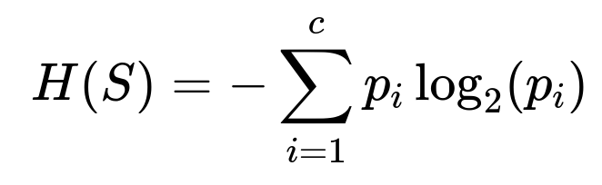
In a decision tree setting:
A leaf node containing only positive or only negative examples has H(S)=0 (no uncertainty).
A node containing a 50–50 split of positive and negative classes has H(S)=1 when c=2 (maximum uncertainty for a binary problem).
Information Gain


Application in Decision Trees
When constructing a decision tree:
At each node (starting from the root), we compute the Information Gain for each candidate feature.
We select the feature that yields the highest Information Gain (i.e., the greatest reduction in entropy).
We partition the data based on this feature and create child nodes.
We recursively repeat this process for each child node until the stopping criteria (such as reaching a maximum depth or having no more features to split) are met, or until all examples in a node are pure (i.e., zero entropy).
Because entropy and Information Gain rely on the distribution of class labels, they are intimately connected to how well a feature can split the data. A feature that splits the data into subsets that each have predominantly one class label will yield a large drop in entropy (and thus a high Information Gain).
Below is a minimal Python code snippet to illustrate how to compute entropy and Information Gain manually for a simple dataset. Though in practice, libraries like scikit-learn handle these computations internally:
import math
from collections import Counter

def entropy(data):
    label_counts = Counter(data)
    total = len(data)
    ent = 0.0
    for label, count in label_counts.items():
        p = count / total
        ent -= p * math.log2(p)
    return ent

def information_gain(parent, children):
    total = sum(len(child) for child in children)
    weighted_entropy = 0.0
    for child in children:
        weighted_entropy += (len(child) / total) * entropy(child)
    return entropy(parent) - weighted_entropy

# Example usage:
parent_data = ["cat", "cat", "dog", "cat", "dog"]  # The 'class' labels
# Suppose we split the data into two subsets based on some attribute
child_1 = ["cat", "cat"]      # Subset for value v1
child_2 = ["dog", "cat", "dog"]  # Subset for value v2

print("Parent Entropy:", entropy(parent_data))
print("Information Gain:", information_gain(parent_data, [child_1, child_2]))
Because decision trees split on the attribute yielding the highest Information Gain, each split tries to isolate classes effectively, leading to a structure that predicts class labels by traversing from the root to a leaf.
Below are possible tricky follow-up questions that often arise in FANG-level interviews, along with detailed answers:
How does entropy compare to other splitting criteria like Gini Impurity?
Entropy and Gini Impurity are both measures of impurity used in decision trees. Entropy comes from information theory and can be interpreted in terms of the expected information (bits) required to classify a sample. Gini Impurity is another measure of how often a randomly chosen element from the set would be mislabeled if it were randomly labeled according to the distribution in the set. In practice:
Entropy tends to penalize heavily when distributions are strongly skewed, while Gini has a smoother response.
They both often yield very similar splits, and the empirical performance difference tends to be small.
Gini Impurity is somewhat faster to compute since it does not involve computing a logarithm, though modern hardware makes this difference usually negligible.
A subtle consideration:
Decision trees that use Gini Impurity are typical of CART (Classification And Regression Trees).
ID3 uses Information Gain (with entropy).
C4.5 also uses Information Gain but incorporates additional adjustments like Gain Ratio to correct for biases toward attributes with many distinct values.
What is Gain Ratio, and why might we prefer it over Information Gain in some cases?
Although Information Gain is straightforward and effective, it can be biased toward features that have many distinct values. For example, a feature that is unique for each sample (like an ID) would split the data perfectly, yielding a high Information Gain but leading to overfitting. Gain Ratio addresses this bias by normalizing the Information Gain by the “split information,” which captures how broadly and uniformly the attribute splits the data.
The “split information” is defined similarly to entropy but applied to how the data is split among the possible values of the feature itself, rather than on the class distribution. By dividing Information Gain by this measure, you get the Gain Ratio, which typically penalizes features with many distinct values. In certain real-world scenarios with high-cardinality features, Gain Ratio can help mitigate overfitting and yield more generalizable trees.
How do we handle continuous or numerical features when computing Entropy and Information Gain?
Decision trees can handle continuous features by identifying thresholds that best split the data. For example, if we have a numerical feature such as “age,” the algorithm tries candidate thresholds (e.g., “age < 30” vs. “age ≥ 30”) to partition the data and computes the resulting Information Gain for each threshold. Then it picks the threshold with the highest Information Gain. Concretely:
Sort the values of the feature.
Evaluate possible split points (often midpoints between consecutive sorted values).
For each split point, divide the data into two subsets and calculate the Information Gain.
Select the split point that yields the highest Information Gain.
A subtlety with continuous features is that you need to re-evaluate thresholds at each step. This can be computationally expensive for large datasets or many continuous features. Many libraries optimize this process by using median-based splits, approximate methods, or randomized thresholds.
Why is Entropy sometimes said to be “slower” to compute than Gini?

Is it possible for Information Gain to be zero for a split?
Yes. If an attribute does not help partition the data into more homogeneous subsets—meaning the subsets have the same class distribution as the original set—then the resulting expected entropy will be the same as the original. Therefore, the Information Gain is zero. In other words, the attribute does not reduce any uncertainty about the class labels.
A hidden pitfall can occur in real-world datasets with many noisy features that provide no real discriminative power. For such features, the best possible split might barely reduce entropy at all, so the computed Information Gain ends up close to zero.
How do missing values affect the calculation of Entropy and Information Gain in practice?
In real-world datasets, missing data is common. Some strategies include:
Ignoring (or removing) the samples that have missing values for the attribute being tested. However, this may cause loss of valuable information.
Imputing missing data using statistical or predictive methods (mean, median, most frequent class, or even more advanced imputation techniques).
Using “branch fraction” methods where a sample with a missing attribute value is fractionally associated with each child node in proportion to how frequently the non-missing samples go to each node. This approach is more complex but can yield more robust trees.
Any approach must be consistent throughout the training and inference process. Failure to handle missing values systematically can degrade both the accuracy and interpretability of the final model.
Could you walk through a small worked example that demonstrates how Entropy and Information Gain drive the first split?
Imagine a tiny dataset of binary class labels ("Yes" or "No") along with an attribute “Weather,” which can be “Sunny” or “Rainy.”
Suppose the dataset is:
6 samples: ["Yes", "Yes", "No", "Yes", "No", "No"]
The corresponding "Weather" labels: ["Sunny", "Sunny", "Sunny", "Rainy", "Rainy", "Rainy"]
Compute overall entropy of the class labels:
Let’s say we have 3 “Yes” and 3 “No.” The probability for each class is p(Yes)=0.5, p(No)=0.5.


Numerically, each subset’s entropy might be around 0.9183 bits (they are symmetric).
Weighted entropy after splitting:

Interpretation:
Splitting on “Weather” gives us some (relatively small) reduction in uncertainty in this artificial example. If we had another feature that split the data into more homogeneous subsets, we would see a higher Information Gain. The tree-building algorithm would compare the IG for all candidate features and choose the one that yields the highest IG at each node.
This example shows how to systematically compute and interpret Entropy and Information Gain in a straightforward manner.
Do decision trees using Entropy and Information Gain tend to overfit?
Decision trees are prone to overfitting if allowed to grow without constraints. Overfitting happens when the tree starts to memorize specific patterns and noise in the training set rather than learning generalizable rules. Common strategies to avoid overfitting include:
Pruning: stopping the tree from growing after a certain depth, or post-pruning by removing less informative splits once the full tree is built.
Setting minimum samples per leaf.
Setting a maximum depth.
Setting a minimum Information Gain threshold for a split.
Using Entropy vs. Gini does not directly solve overfitting, because both metrics will keep splitting as long as they can reduce impurity. Hence, we rely on the regularization techniques mentioned.
How might you explain these concepts to a non-technical stakeholder?
While a non-technical stakeholder may not need the precise formula, they can grasp it via analogy:
Think of Entropy as measuring how “mixed up” a basket of fruits is. If you have a basket with only apples, it’s very ordered (low entropy). If you have apples, oranges, bananas, all in roughly equal amounts, it’s very “mixed up” (high entropy).
Information Gain is how much you reduce the “mixed up” nature by splitting the basket based on some attribute (e.g., color). If sorting by “color” isolates apples from oranges and bananas, you’ve significantly reduced the confusion, gaining valuable information.
Such analogies can help non-technical collaborators understand why certain splits are chosen and how the concept of “uncertainty reduction” underpins the decision tree approach.
How does this relate to model interpretability?
One of the biggest advantages of decision trees is their interpretability. Each node in the tree corresponds to a particular split on a feature. Because we rely on Information Gain (driven by entropy) to choose the splits, the resulting path from the root to a leaf can be read off like a series of understandable rules, for example:
If Age < 30 and Income ≥ 50k → Class = “Likely to buy.”
If Age ≥ 30 → Class = “Unlikely to buy.”
In interviews, you might be asked to compare this interpretability to that of other models. Decision trees are typically easier to interpret than neural networks or ensemble methods, but they can become less interpretable if they grow very large. Techniques like post-pruning can make them smaller and thus more interpretable.
How do these concepts generalize to multiple classes?
Entropy naturally extends to multi-class classification by summing over each of the c classes. The formula does not change other than having more terms. Information Gain then uses the same definition, but again the entropy sums across all classes. The principle remains: find the split that maximally reduces the overall entropy of the node.
In real-world multi-class scenarios:
We might have features that do a great job separating one specific class from the rest, resulting in a big drop in entropy. That feature typically emerges as having high Information Gain.
The question of how to handle continuous vs. categorical features remains, but the computations simply extend to the multi-class probabilities.
Could using Entropy lead to any specific biases in the splits chosen?
In practice, Entropy can sometimes favor splits that isolate very small pure subsets, especially if that yields a big local reduction in uncertainty. If your dataset has highly unbalanced classes or some features with many unique values, standard Information Gain might be biased in ways that do not generalize well (this is the reason for Gain Ratio in algorithms like C4.5).
Also, if the dataset has a large class imbalance, the entropy measure could be skewed if not interpreted carefully. It’s often beneficial to look at actual distributions in each node and apply domain knowledge rather than relying purely on entropy calculations. Pruning or setting minimum child node sizes can help mitigate these biases.
Summary of the Core Ideas
Entropy provides a foundation for measuring how “mixed” a set of class labels is, and it captures the uncertainty present in the data. Information Gain quantifies how much entropy is reduced by splitting on a particular feature. In building a decision tree, features are chosen based on the highest Information Gain (or a related criterion like Gain Ratio), thereby recursively partitioning the dataset until it reaches homogeneous (or sufficiently small) subsets. Although decision trees can overfit if not properly controlled, the notion of reducing entropy at each step remains central to their interpretability and effectiveness.
By understanding these quantities and the subtle ways in which they can be computed, interpreted, and potentially biased, practitioners can build more robust decision trees. They can also communicate effectively to diverse stakeholders about why a particular decision tree model makes the splits that it does.
Below are additional follow-up questions
Could there be scenarios where a locally optimal split (based on Information Gain) leads to suboptimal overall tree performance?
When building a decision tree via Entropy and Information Gain, each node’s split is determined in a greedy manner: the feature that reduces entropy most at that node is chosen. However, this local optimum does not always result in a globally optimal tree.
Detailed Reasoning
Greedy Nature: At any node, we pick the split with the highest immediate Information Gain. This does not factor in how future splits might interact. There could be a situation where a split with slightly lower Information Gain at an earlier node enables greatly improved splits down the line, resulting in a better overall tree.
Search Space: Decision tree algorithms typically do not perform an exhaustive search over all possible tree structures because the search space grows exponentially with the number of features. A fully optimal solution (in terms of minimal classification error) would require searching across all possible trees, which is usually infeasible.
Real-World Pitfall: In practice, a locally optimal choice might cause the next splits to be less effective. For example, if an early split isolates a subset of data that appears pure but actually contains subtle patterns requiring further splits, the local greedy choice might hamper a more nuanced separation later.
Mitigation Strategies
Pruning: Either pre-prune (decide not to split if the Information Gain is below a threshold) or post-prune (build a large tree and then prune back) to improve generalization.
Ensembling: Methods like Random Forests and Gradient Boosted Trees aggregate multiple (often smaller) decision trees to reduce the risk of a single, suboptimal split dominating the outcome.
How do highly correlated features influence the splits chosen by Information Gain?
In real-world datasets, features can be correlated. For instance, “height in centimeters” and “height in inches” measure the same underlying concept, just in different units. Decision tree splits based on Information Gain may behave unexpectedly in such situations.
Detailed Reasoning
Redundant Splits: If two features are strongly correlated, the algorithm might choose one of them at the top node because it has the highest Information Gain. Then, when considering further splits, the second correlated feature becomes less informative—its marginal Information Gain is lower because the first split already captured most of the shared variance.
Overfitting Concern: Sometimes, correlated features can lead to repeated, slightly different splits that over-segment the data. For example, if the tree first splits on “height in cm,” a subsequent split on “height in inches” might not add real new information but can overfit to tiny variations in the data.
Multicollinearity: Although multicollinearity is more commonly discussed in linear models, in decision trees it can still distort the relative importance assigned to each feature, especially if the dataset is small.
Pitfalls and Practical Considerations
Feature Selection: You can reduce correlation by removing redundant features or transforming them (e.g., principal component analysis) if they are highly collinear. This sometimes yields simpler trees.
Regularization: Depth limitations and minimum-sample-per-split constraints can prevent the tree from over-splitting on correlated features.
What is the effect of large numbers of categories in a single categorical feature on Information Gain?
Large categorical features (sometimes called “high-cardinality” features) can pose unique challenges in decision tree splits using Entropy and Information Gain.
Detailed Reasoning
Potential Overfitting: A categorical feature with many distinct values might create splits that isolate very small subsets of data. This often leads to artificially high Information Gain for that feature, particularly if any subset becomes pure by happenstance.
Biased Splits: Similar to the rationale for using Gain Ratio, a feature with many categories can produce a misleadingly large reduction in entropy. For instance, a feature like “user_id” might appear to perfectly separate samples—each user_id is unique—but it offers no real predictive power on unseen data.
Practical Challenges: Decision trees that do not handle large categorical features carefully might spawn huge branching factors, making the tree overly complex and less interpretable.
Possible Solutions
One-Hot Encoding or Target Encoding: Converting a large categorical feature into multiple binary features or using mean target encoding can help. Though, these transformations must be done with caution to avoid data leakage or explosion in dimensionality.
Regularization: Some implementations limit the number of categories a tree node can split on or apply advanced techniques like binning categories by their frequency or by estimated class distribution.
How does data scaling or transformation interact with Entropy and Information Gain for continuous features?
Unlike algorithms that rely on distance metrics, decision trees using Entropy/Information Gain typically do not require normalization or standardization. Still, data transformations can occasionally affect split thresholds or the distribution of data in non-obvious ways.
Detailed Reasoning
Threshold Identification: For a continuous attribute, the algorithm tries thresholds between sorted feature values. Whether the feature is scaled from 0 to 1 or measured in large integers typically does not change the relative ordering. Therefore, the potential split points remain at the same positions in the sorted list, preserving Entropy-based splits.
Edge Cases: If a transformation (e.g., logarithmic transform) significantly changes the distribution shape (like compressing a skewed feature), the best threshold for a split might change. This can lead to different subsets of data being isolated, potentially altering the tree structure.
Correlated Effects: If multiple features are strongly skewed and you apply transformations differently to each, it can unexpectedly reduce or accentuate correlations, influencing how the tree chooses splits.
Practical Tips
Minimal Impact if Order is Preserved: Scaling that preserves feature ordering (e.g., min-max scaling) will not typically change which threshold yields the best Information Gain.
Reshaping Distributions: Non-linear transformations (e.g., log(x+1)) that reshape distributions can yield different thresholds and sometimes improve model performance if the original scale was very skewed.
In what ways do floating-point precision issues impact Entropy and Information Gain in large datasets?
When dealing with large datasets or when class distributions are very skewed, floating-point arithmetic can become a hidden challenge in computing Entropy and Information Gain.
Detailed Reasoning

Summations and Subtractions: Information Gain is the difference between entropies. Subtraction of nearly equal floating-point numbers can lead to “catastrophic cancellation,” where significant digits are lost and the result becomes less accurate.
Practical Relevance: Though in most typical machine learning tasks these errors are small and do not drastically change which split is chosen, in some edge cases with extremely large data or extremely unbalanced classes, the numerical stability might affect early splits or certain tie situations.
Mitigation
Stability Techniques: Libraries often implement stable log-sum-exp or other numerically robust methods.
Data Binning: For extremely large data, sometimes using approximate histograms or binning reduces the resolution at which probabilities are calculated, improving numerical stability while retaining an accurate enough estimate of entropy.
How is Shannon entropy in decision tree learning related to the original concept of entropy in information theory?
Entropy in decision trees stems directly from Shannon’s definition in information theory, where it measures the average information content or uncertainty of a random variable.
Detailed Reasoning
Same Formula: The formula for Shannon entropy,

Interpretation: In information theory, entropy quantifies the expected number of bits needed to encode the outcome of a random variable. In a decision tree context, it reflects how many bits are needed on average to describe the class of a randomly chosen sample from the dataset.
Connection to Information Gain: “Information Gain” in tree learning parallels the concept of “mutual information” in information theory—how many bits of uncertainty are removed about the class label by observing a particular feature.
Real-World Insights
This direct link to information theory lends an intuitive foundation for why we measure data “impurity” with entropy: the more uncertain (mixed) it is, the higher the “cost” (in bits) to label a point.
What strategies exist for selecting thresholds in continuous features more efficiently when the dataset is huge?
Traditional decision tree algorithms often evaluate all possible thresholds (or all midpoints between sorted values) for continuous features, which can be computationally expensive for massive datasets.
Detailed Reasoning
Linear Scan: The naive approach is to sort the values once and try candidate thresholds between consecutive unique values. If a feature has nn unique values, this yields up to (n−1) potential splits. For large n, this can be very slow when repeated for many features.
Approximate Methods: Some libraries, such as XGBoost or LightGBM, create histograms of feature values and evaluate a smaller set of candidate thresholds based on bin centers or boundaries. This approach substantially lowers computational overhead at the cost of minor approximation error in the Information Gain calculation.
Quantile Binning: Another approach is to select thresholds at certain quantiles of the distribution (e.g., deciles or percentiles). This ensures that each bin (interval) roughly contains the same number of samples, reducing the total number of thresholds to consider.
Practical Considerations
Trade-off: Fewer thresholds mean faster training but potentially less precision in capturing the best split point. For large-scale problems, the small loss in precision is often outweighed by the significant speed gain.
How does the choice of logarithm base (e.g., base 2 vs. natural log) affect Entropy and Information Gain?
In the standard definition, Entropy commonly uses a base-2 logarithm. However, one could use a different base, such as the natural logarithm. The result is just a constant scaling factor.
Detailed Reasoning

Interpretation in Bits vs. Nats:
Base-2 implies the information is measured in bits.
Using the natural log implies measuring in nats. Despite different units, the direction of improvement in entropy reduction does not change.
2. Common Practice: Most ML textbooks and frameworks default to base-2 for interpretability in terms of bits. Implementation details might use natural logs, especially if they rely on common math libraries that default to e-based logs.
Result The choice of log base does not affect which feature is considered optimal for a split or the structure of the tree. It merely changes the scale on which Entropy and Information Gain are reported.
What are common failure modes if your dataset is extremely small or extremely noisy?
Small datasets and noisy data can cause decision trees using Information Gain to exhibit pathological behaviors.
Detailed Reasoning
Overfitting in Small Datasets: With very few samples, each split can drastically reduce the sample count in child nodes, pushing them toward artificially low entropy (pure subsets). This leads to a high-variance model that does not generalize well.
Noise or Mislabels: If the dataset contains mislabeled samples or random fluctuations, the algorithm might identify spurious splits that perfectly isolate those noisy points, again inflating Information Gain in a misleading way.
Insufficient Representation: For a small dataset, having many features can cause some splits to look very good purely by chance, especially if the features have many unique values.
Possible Remedies
Gather More Data: Ideally, increasing dataset size to reduce variance.
Regularization and Pruning: Prune aggressively or enforce a minimum number of samples per split.
Data Cleaning: Identify and correct mislabeled points or outliers if possible.
Does the method of handling ties in Information Gain matter, and how is it implemented?
Sometimes, two or more features yield exactly the same Information Gain. This tie can occur for multiple reasons, including symmetrical features or numerical coincidences.
Detailed Reasoning
Tie-Breaking Mechanisms: In practice, libraries might break ties in different ways—some might pick the feature that appears first in the dataset’s feature list, others might pick randomly among features that yield the same gain, or apply additional criteria like Gain Ratio or the number of distinct values.
Impact on Tree Structure: Different tie-break strategies can result in slightly different tree structures, even though the final accuracy might be similar. Over many splits, these small variations might compound into somewhat different models.
Edge Case: In extremely balanced datasets or ones where certain features are duplicates or symmetrical, tie situations could recur often, making tree construction sensitive to tie-break rules.
Practical Tips
If reproducibility is crucial, fix a random seed or use a consistent tie-breaking policy to ensure the same splits.
Investigate if repeated ties indicate redundant or correlated features. Possibly remove or combine them.