ML Interview Q Series: Practical Feature Selection and Dimensionality Reduction for High-Dimensional Datasets.

📚 Browse the full ML Interview series here.

Feature Selection in Practice: Imagine you have a dataset with thousands of features, but you suspect many of them are irrelevant or redundant. What techniques could you use to perform feature selection or dimensionality reduction before modeling? Provide examples such as removing features with many missing values, using filter methods (e.g., based on correlation or mutual information), wrapper methods (recursive feature elimination), embedded methods (lasso or tree-based feature importance), or using PCA to reduce dimensionality.

Feature Selection and Dimensionality Reduction are both crucial steps for addressing large feature spaces, especially when we suspect many features are irrelevant, redundant, or noisy. The main reasons include improving model generalization, reducing overfitting, and decreasing computational costs. Below is a thorough discussion of the approaches.

Feature Selection generally focuses on choosing a subset of the original features. Dimensionality Reduction typically transforms the original features into a fewer number of latent variables (like in PCA). Although the line can blur between the two, the distinction is that feature selection keeps actual features (or a subset of them) while dimensionality reduction creates new, lower-dimensional representations.

Feature selection can be organized into these categories:

Filter Methods Wrapper Methods Embedded Methods

In addition to those, we often use PCA or other methods for dimensionality reduction.

Removing Features With Many Missing Values can also be seen as a preliminary step for data cleaning, but in practice, it can function as an initial form of feature selection.

Feature selection approaches are often combined: for instance, you might first remove features with too many missing values or zero variance, then apply a filter-based correlation threshold, and finally use a wrapper or embedded method to refine the final subset.

Removing Features With Many Missing Values It is common to remove features that have too little information. If a feature has, for example, more than 90% of its values missing, it may be safer to discard it altogether unless there is a compelling reason to keep it. This avoids complicated imputation and the risk of introducing large biases or noise. A typical approach is to set a missing-value threshold. For instance, if a feature is missing over a certain percentage of values, drop it. After dropping those features, we handle the remaining missing data with suitable techniques (e.g., mean/median imputation, or more sophisticated methods like KNN imputation).

Filter Methods These rely on statistical measures of relevance between each feature and the target variable. Filter methods do not consider interactions between features directly (except in specialized forms like advanced correlation analysis). Some popular filter methods:

Correlation Filtering One standard approach is to compute correlation coefficients (e.g., Pearson correlation) between each feature and the target for regression tasks, or something like the point-biserial correlation for classification tasks with binary targets. If the absolute correlation is below a predefined threshold, or if it is extremely high with other features, it might indicate that feature can be removed. It is also common to look at pairwise correlations among features. If two features are strongly correlated, we might remove one of them to reduce redundancy.

Mutual Information Mutual information measures the amount of information that two variables share. The formula (in an informal sense) is:

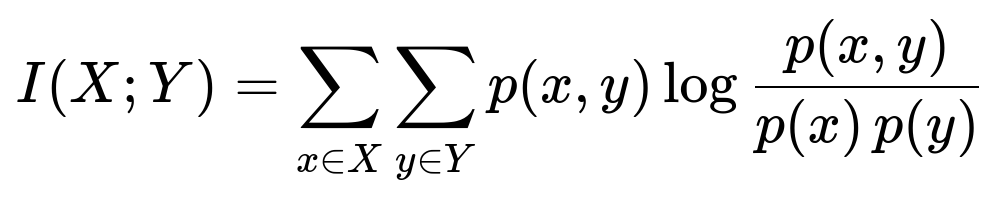
Intuitively, mutual information tells us how much knowing one variable reduces uncertainty about the other. If the mutual information between a feature and the target is low, that feature may be less relevant. Compared with correlation, mutual information can capture some non-linear relationships between the feature and the target. This is especially helpful for classification problems with categorical features or for capturing more complex relationships.

Statistical Tests For classification tasks, we might use chi-square tests or ANOVA F-tests to see how strongly a feature relates to the target. Typically, a high chi-square statistic (for categorical features) or a high F-statistic (for continuous features in a classification scenario) indicates the feature is quite relevant to predicting the target.

Wrapper Methods Wrapper methods use the model’s performance (e.g., cross-validation accuracy) to select features. The idea is to wrap the model training inside a search procedure to find the best subset of features. This can be more computationally expensive, especially with thousands of features, but it generally finds a subset more specifically tailored to the model of interest.

Recursive Feature Elimination (RFE) A common wrapper approach is RFE. We start by training a model (often a linear or tree-based model) on all features, ranking features by their importance or coefficients, and then removing the least important features. We repeat until we reach a desired number of features. This can be slow for very large datasets, especially if the model is computationally heavy. But it tends to deliver strong results because it directly uses the model’s view of importance.

Exhaustive Search Methods One might attempt a brute force or stepwise approach (forward selection or backward elimination) but this is often infeasible for thousands of features because the number of possible subsets is astronomically large. Hence, RFE or other heuristics are more popular.

Embedded Methods These methods rely on the model itself having a built-in way to perform feature selection. Common examples:

Lasso ( Regularization) Lasso is a regression method that adds an penalty on the absolute values of coefficients:

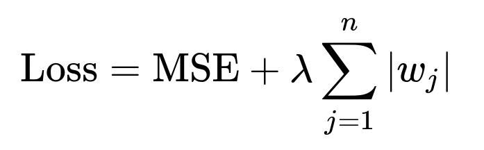
Because the penalty tends to shrink some coefficients to zero, it effectively excludes less important features from the model. This property makes lasso an attractive embedded feature selection method for regression tasks.

Elastic Net Elastic Net is a mix of and regularization. It can also zero out coefficients and helps when features are strongly correlated with each other, which can cause instability in a purely method. This is a robust approach for high-dimensional data.

Tree-Based Models Tree-based methods (e.g., Random Forest, Gradient Boosted Decision Trees) compute feature importance based on measures like Gini importance or information gain. These importances can be used to select a subset of top-ranked features. Feature importances from ensemble models are generally more robust than from a single Decision Tree. However, one must be cautious if the dataset is heavily unbalanced or if some features have many unique values, as that can bias the importance metrics.

Dimensionality Reduction with PCA PCA (Principal Component Analysis) is not strictly a “feature selection” method. It transforms the original features into orthogonal principal components. By keeping only the first few components explaining most of the variance, we effectively reduce dimensionality. In mathematical form, PCA finds directions (principal components) that maximize variance. The steps:

1. Center the data (subtract mean).

2. Compute the covariance matrix.

3. Find eigenvalues and eigenvectors of that covariance matrix.

4. The top principal components are those associated with the largest eigenvalues.

We can then retain the top k components, typically chosen to explain a certain percentage (like 90% or 95%) of the variance in the data. This approach can drastically reduce dimension in a continuous feature space.

Use Cases for Each Technique When we want to retain interpretability of original features, we usually go with feature selection (filter, wrapper, or embedded). When interpretability is less of a priority but we need powerful dimensionality reduction, PCA or other transformations (like t-SNE for visualization, or autoencoders in deep learning) may be used.

Practical Implementation Example (Python)

import pandas as pd
import numpy as np
from sklearn.feature_selection import RFE, SelectKBest, mutual_info_classif
from sklearn.linear_model import LogisticRegression
from sklearn.ensemble import RandomForestClassifier
from sklearn.decomposition import PCA

# Suppose df is your DataFrame, and 'target' is the column name for the label
X = df.drop(columns=['target'])
y = df['target']

# 1) Remove features with too many missing values
threshold = 0.9
missing_fraction = X.isnull().mean()
X = X.loc[:, missing_fraction < threshold]

# 2) Simple Filter: Use mutual information to pick top features
selector = SelectKBest(mutual_info_classif, k=50)  # keep top 50
X_selected = selector.fit_transform(X, y)

# 3) Wrapper: RFE with Logistic Regression
model = LogisticRegression(max_iter=1000)
rfe = RFE(estimator=model, n_features_to_select=20, step=1)
rfe.fit(X_selected, y)
# The boolean mask of selected features
rfe_mask = rfe.support_

# 4) Embedded: Feature Importances from Random Forest
rf = RandomForestClassifier(n_estimators=100)
rf.fit(X_selected, y)
importances = rf.feature_importances_
# Sort features by importance and choose threshold or top-n

# 5) PCA Dimensionality Reduction
pca = PCA(n_components=10)
X_pca = pca.fit_transform(X.fillna(X.mean()))  # fill missing with mean for demonstration

In this code snippet, we combined multiple steps. In practice, you would tailor these to your problem, possibly in a pipeline that handles missing values and scaling in a well-structured manner.

Potential Pitfalls to Keep in Mind Some methods are biased by specific data distributions, outliers, and scale. For example, correlation-based filtering is not always the best for non-linear relationships. Also, applying PCA blindly can lose interpretability. Overfitting in wrapper methods with small data is another risk, so cross-validation is key. Additionally, if your data has strong domain constraints or domain knowledge, incorporate that to guide which features to drop or keep.

What if the number of features is extremely large?

For extremely large feature spaces (e.g., tens or hundreds of thousands of features), we often do the following:

• Use high-throughput filter methods (like correlation or mutual information) to discard a vast majority of unhelpful features quickly.

• Use more computationally expensive methods (like RFE or embedded methods) only on a smaller subset that survived the initial filtering step.

• Consider domain-driven feature grouping or hashing techniques for extremely high-dimensional text data, for example.

• Use specialized dimensionality reduction methods tailored to the domain (like topic modeling for text, or embedding-based approaches in deep learning).

Follow-up Questions

How does one decide between filter, wrapper, or embedded methods in practice?

Each has different trade-offs. Filter methods are fast and are a good first pass to eliminate clearly irrelevant features. Wrapper methods, especially RFE, can be more accurate since they test actual model performance. However, they can be computationally expensive. Embedded methods strike a balance by leveraging regularization or model-based feature importance internally. In practice, one might start by applying filter methods to reduce the feature set size, then apply a wrapper or embedded method on the reduced set. This approach preserves the interpretability and the strong link with actual model performance.

Additionally, consider the type of model you plan to deploy. If you are using a linear model with regularization (like Lasso), the embedded approach is straightforward. If you plan on using tree-based ensembles, computing feature importances is a natural embedded approach. If the dataset is massive, filter methods might be your only practical approach for an initial pass.

Can you explain how to handle features that have high correlation among themselves?

High correlation among features can lead to multicollinearity issues. A simple approach is to measure pairwise correlations among features and, if two features exceed a certain threshold (e.g., 0.9), drop one. Doing so helps reduce redundancy and can stabilize model training. Alternatively, a tree-based method might naturally down-weight one correlated feature. But for linear models, correlated features can inflate variance in the coefficient estimates. This is why regularization (ridge) helps in correlated feature settings by shrinking coefficients. In summary, you either drop one or more correlated features in a filter step, or rely on a model-based approach (like Lasso, Ridge, or a tree ensemble) to handle correlation.

Is PCA always the best way to do dimensionality reduction?

PCA is one of the most widely used linear dimensionality reduction techniques, but it might not capture non-linear structures in the data. If the data has complex non-linear manifolds, more advanced methods like Kernel PCA, t-SNE (for visualization), or autoencoders might reveal richer structure. Also, PCA can obscure interpretability since the new components are linear combinations of the original features. If interpretability is crucial, you might stick to feature selection. If your goal is purely to improve model accuracy or compress data, PCA (or other transformations) may be very effective.

What is the relationship between scaling and PCA?

PCA is sensitive to the scale of different features. By default, features with larger variances tend to dominate the principal components. Therefore, standard practice is to scale or standardize features before applying PCA. Typically, you subtract the mean and divide by the standard deviation of each feature. This ensures that PCA does not overweight features that inherently have a larger scale.

If a feature has many missing values, is it always best to remove it?

Not necessarily. Sometimes, a feature with many missing values might be extremely predictive because the very fact that data is missing could convey signal (for instance, in certain medical tests, if the value was not measured because a patient refused or a test was not necessary, that might implicitly correlate with an outcome). Instead of outright removing features with excessive missingness, you can engineer “missingness indicators” (binary flags) that record whether the feature was missing or not. Then you can try various imputation strategies (mean, median, MICE, KNN, or domain-specific methods). But if there is no strong rationale, or if the missingness is purely random, removing the feature might be simpler.

How do I verify that feature selection actually improves my model?

The best way is through rigorous cross-validation. Compare the performance of the model with and without feature selection using the same cross-validation splits. If you are applying a method like RFE, it is usually integrated with cross-validation from the start to avoid overfitting to one particular training set. You might see improved generalization, simpler models, fewer correlated errors, and faster inference. If performance is the same or better with fewer features, that is generally a win. If performance drops severely, you need to reevaluate your approach.

Is it okay to apply the feature selection on the entire dataset before splitting into train and test?

It is best practice to include the feature selection step inside a cross-validation pipeline, so that feature selection is fit only on the training folds and not on the test fold. If you fit the selection step on the entire dataset first, you might inadvertently leak information from the test set. This results in overly optimistic estimates of generalization performance. Therefore, we typically do:

1. Split data into train and test (and possibly further into folds if doing cross-validation).

2. Within each training fold, perform feature selection (like RFE, filter, or embedded) and then train the model.

3. Evaluate on the corresponding validation fold.

4. After cross-validation, finalize the set of features or the pipeline.

5. Retrain on the entire training set using that pipeline (including feature selection) and evaluate on the held-out test set.

What if we have categorical features as well? How do we handle them in feature selection?

Categorical features require special treatment. For filter methods based on correlation, you might encode them (e.g., one-hot encoding) and then check correlation among the encoded dummy variables. Or you can use mutual information or chi-square tests, which often work directly with categorical variables. For wrapper and embedded methods, you can feed them as you normally would to the model (with an appropriate encoding like one-hot). Tree-based models handle categorical features well if they are suitably encoded, and they yield importance measures. For lasso or logistic regression with regularization, you typically have to one-hot encode, so that naturally splits each categorical feature into multiple binary features. In such scenarios, the regularization can zero out entire sets of dummy variables if they are less informative.

How do advanced neural-network-based approaches fit into the dimensionality reduction or feature selection discussion?

Deep learning methods sometimes perform a kind of “feature extraction” from raw high-dimensional inputs. For example, an autoencoder can be used for dimensionality reduction by compressing the input into a lower-dimensional latent space. Another possibility is a network with a bottleneck layer. Once trained, the activations in that layer can be seen as a reduced representation. Feature selection can also be integrated into neural networks through specialized regularizations. For instance, group regularization over input neurons can zero out entire groups of weights associated with less useful features. However, these are less commonly used than standard approaches (like lasso or tree-based methods), because deep learning typically expects abundant data to directly learn relevant representations.

Under what circumstances might you decide not to do feature selection at all?

If your dataset is not large (in terms of the number of features) relative to the number of samples, and if your model is not suffering from overfitting or interpretability issues, you may decide to keep all features. Some models, such as tree-based ensembles with enough regularization, can handle large feature spaces fairly well. Likewise, methods like ridge regression can handle a large number of correlated features. If domain knowledge suggests that each feature might carry some relevant signal, you might keep them all and let the model’s regularization handle any redundancy.

---

Below are additional follow-up questions

How do we handle feature selection when we have multiple output variables (multi-output regression or multi-label classification)?

When the problem involves predicting more than one target variable simultaneously, standard single-output feature selection methods might not fully capture interactions across all targets. In multi-output regression, a set of features could be critical for one target but irrelevant for another. Similarly, in multi-label classification, some features might only be informative for a subset of labels.

One strategy is to apply single-target feature selection methods independently to each target, then take the union or intersection of the selected features. However, this approach may lose synergy among targets. An alternative is to use multi-output models (like some tree-based methods or neural networks designed for multi-output tasks) and rely on embedded feature importance.

Potential pitfalls:

• Over-selecting features for a single output: If certain outputs have high variance or strong signals, they may dominate the feature importance for the entire model.

• High correlation among targets: If your multiple outputs are correlated, some features may be crucial for multiple outputs simultaneously, masking the role of others.

• Complex interpretability: Understanding why a feature is selected in a multi-output context can be more challenging if each target has a different functional relationship to that feature.

Edge cases include settings where some outputs are categorical, some are continuous, or where certain targets have very limited data. In such cases, it might be beneficial to employ flexible embedded methods (e.g., specialized multi-task neural networks or multi-task Lasso-like approaches) that can jointly consider correlations among targets.

Are there any issues that arise when we do feature selection if we suspect distribution shift or domain shift in future data?

When future data is expected to differ from the training distribution, standard feature selection methods risk selecting features that are highly predictive in the historical dataset but may not remain predictive under new conditions. This distribution shift can occur due to changing user behavior, concept drift, or variations in data collection processes.

One approach is to check the stability of feature importance across multiple time windows or across subpopulations. If certain features consistently appear important across diverse samples, they are likely more robust to shifts. Techniques like adversarial validation can also be used to detect if the training and future distributions differ significantly.

Pitfalls:

• Overfitting to past data: A feature may be extremely predictive in old data but loses significance when conditions change.

• Ignoring domain knowledge: If domain experts anticipate certain features will shift in meaning or scale, purely data-driven selection might fail to account for that.

• Scarcity of future data: Often, you do not have a substantial dataset from the new domain, so validating the robustness of selected features is difficult.

Edge cases involve rapidly evolving contexts—like user behavior on social media—where the target’s meaning and the predictive power of features can change drastically in a short period. In such scenarios, periodic re-selection of features or model updates might be necessary.

How should we handle feature selection if we have noisy labels or uncertain target data?

Noisy labels (i.e., cases where the observed target might be partially wrong or corrupted) can degrade the fidelity of any supervised method, including feature selection. Traditional filter methods that rely on correlation or mutual information with the noisy target may select spurious features. Wrapper methods can also be misled during cross-validation.

Possible strategies:

• Robust methods: Regularized models, such as Ridge, Lasso, or robust tree ensembles, can partially mitigate label noise by controlling overfitting.

• Re-labeling or label cleaning: If feasible, check questionable labels or gather additional label sources to improve label accuracy.

• Noise-aware weighting: If you know certain samples have higher confidence labels, weigh them more in the feature selection process.

Pitfalls:

• Selection of “noise-fitting” features: A strongly overfit model might pick up random correlations that only exist in mislabeled examples.

• Underestimating truly informative features: If a feature’s signal is drowned out by noise, naive feature selection might exclude it prematurely.

• Data scarcity: If your dataset is small and labels are noisy, it’s doubly hard to distinguish relevant from irrelevant features.

In edge cases where the label itself is uncertain (e.g., in medical diagnoses that might contain subjective elements), methods like multi-instance or multiple-label learning might be more suitable, and feature selection must adapt to these frameworks.

When applying an unsupervised dimensionality reduction technique like PCA or autoencoders, how do we decide how many components or how large the latent dimension should be?

Deciding the number of components in PCA or the dimensionality of an autoencoder’s bottleneck layer often involves a balance between explained variance (or reconstruction error) and the interpretability or practicality of the reduced space.

A typical approach with PCA is to plot the cumulative explained variance and pick the smallest number of components that capture a large fraction (e.g., 90-95%) of variance. With autoencoders, you might monitor reconstruction loss on a validation set, gradually increasing or decreasing the bottleneck size until you find a satisfactory trade-off between performance and dimensionality.

Pitfalls:

• Over-reliance on variance explanations: Capturing 95% of the variance doesn’t necessarily mean capturing 95% of the signal that’s predictive for a target. It only ensures variance in the input space is retained.

• Overfitting: In an autoencoder, too large a latent dimension may simply memorize the data rather than extract meaningful latent factors.

• Loss of interpretability: The more dimensions you keep, the harder it can be to interpret principal components or latent representations.

Edge cases include highly skewed data with outliers—where PCA might dedicate entire components to describing outliers. In such scenarios, robust PCA variants or domain-driven transformations might be preferable.

Could you explain scenario-based feature selection, where we might have different subsets of features for different inference scenarios?

In some real-world applications, we might need different feature subsets for different deployment environments. For example, a company might have a real-time inference pipeline that can only compute a limited set of features quickly, while an offline batch pipeline could incorporate a richer feature set. Scenario-based feature selection tailors the subset of features to each usage scenario.

One way to achieve this is to define constraints (like inference time, memory usage, or data availability) and perform feature selection that respects these constraints. For example, we might run a filter or embedded method with an added penalty for features that are slow or expensive to compute.

Pitfalls:

• Misalignment of training vs. inference: If you train with a large feature set but deploy with fewer features, your model might be less accurate in production.

• Feature drift: Some features might not be available in real time (e.g., user has not completed a specific form yet), which leads to incomplete data.

• Maintenance complexity: Maintaining multiple sets of features across different environments can introduce data consistency issues.

Edge cases occur in low-latency systems (like high-frequency trading) where you might only have milliseconds to generate predictions. The feasible set of features shrinks drastically, requiring specialized real-time feature selection or dimensionality reduction.

How do we interpret the results of a selected feature set if the model is highly complex, like gradient boosting or deep neural networks?

Complex models often act as “black boxes,” making it challenging to glean how each selected feature contributes to predictions. Even after you select features, the relationships between these features and the output can be nonlinear and highly interactive.

Strategies for interpretation:

• Permutation importance: After selecting features, measure how much randomizing each feature’s values degrades model performance. A large drop indicates high importance.

• Partial dependence plots (PDP) or individual conditional expectation (ICE): These techniques help visualize how the model’s predictions change as you vary a feature, holding others fixed (in theory).

• SHAP values: SHAP (SHapley Additive exPlanations) can attribute the prediction difference from a baseline to each feature. Even for deep neural networks or boosted trees, approximations can be used to compute SHAP values.

Pitfalls:

• Misinterpreting importance: High importance does not necessarily mean causality—correlation or confounding can still exist.

• Computational overhead: Techniques like SHAP can be expensive with large models or large datasets.

• Overfitting in explanations: If the model is extremely overfit, the interpretability methods might highlight spurious patterns.

Edge cases include ensemble-of-ensembles approaches or very large neural networks where the dimensionality is huge. Traditional interpretability methods may become intractable or produce incomplete pictures, requiring domain-driven interpretability checks.

How do we handle scenario where we have extremely unbalanced data or extremely rare events for some features?

For classification tasks with extreme class imbalance (such as fraud detection or rare disease diagnosis), many filter and wrapper methods focus on overall accuracy or correlation measures that can be misleading. A feature that is highly predictive of rare events could still appear unimportant if most of the dataset belongs to the majority class.

Possible approaches:

• Customized metrics: Instead of accuracy or standard correlation, rely on metrics relevant to class imbalance (e.g., precision-recall AUC, F2-score, or cost-sensitive measures).

• Data sampling strategies: Oversample the minority class or undersample the majority class in a way that preserves important relationships, then perform feature selection. Synthetic data generation (SMOTE) can also help, though it may alter feature distributions.

• Embedded methods with class-weighting: Tree-based models or linear models can be given higher weight for minority-class examples, thus altering how feature importances or coefficients are learned.

Pitfalls:

• Ignoring sample size: If the minority class is extremely small, even advanced sampling might not produce a stable measure of a feature’s relevance.

• Over-synthetic sampling: Generating many synthetic points can cause the feature selector to learn spurious patterns.

• Operational cost: If the cost of missing a positive (rare event) is very high, your selection should emphasize recall or sensitivity for that class.

Edge cases include multi-class scenarios where multiple classes are each small in proportion. Traditional binary imbalance handling might not directly extend, requiring custom rebalancing strategies or cost matrices.

How do we handle feature selection if the data is highly sparse, such as text classification or extensive one-hot encoding?

When dealing with sparse inputs (like one-hot-encoded text features, high-dimensional user interactions, or large-scale categorical data), feature vectors can have thousands or millions of dimensions, most of which are zeros. Filter-based methods (like mutual information) and embedded methods (like -regularized linear models) are particularly appealing here because they scale well and can zero out irrelevant features.

Typical processes:

• Sparse vectorization: Use TF-IDF or hashing-based vectorization for text, then a filter method (e.g., keep terms with high variance or high mutual information).

• Embedded methods: A Lasso or sparse logistic regression can drastically reduce the feature set by pushing many weights to zero.

• Dimensionality reduction for text: Techniques like truncated SVD (sometimes called LSA—Latent Semantic Analysis) can transform sparse text data into a dense, lower-dimensional representation.

Pitfalls:

• Loss of interpretability: If you rely on hashing or SVD, you lose direct interpretability of which tokens/words remain relevant.

• Memory constraints: Even storing extremely large sparse matrices can be challenging, requiring specialized data structures.

• Over-pruning: If you set regularization too strongly or filter thresholds too aggressively, you might drop moderately useful terms that collectively contribute to the model.

Edge cases involve extremely large corpora where certain domain-specific terms or rare phrases matter a lot. Blindly discarding features that appear “rare” might omit essential clues.

If we are dealing with sequential or time-series data, how do we adapt feature selection or dimensionality reduction methods to account for temporal dependencies?

Time-series data brings the challenge that each observation is not independent; instead, data is correlated over time. Standard feature selection methods may ignore these temporal dependencies, resulting in features that do not generalize well when future time windows shift.

Adjustment strategies:

• Sliding window or lag-based features: Instead of selecting from raw features at a single time point, create multiple lags (like day-1, day-2, day-7 values) for each variable. Then use feature selection to pick which lags matter most.

• Rolling cross-validation: Ensure that the selection process does not leak future information. Perform a rolling window evaluation where training sets are strictly in the past relative to validation sets.

• Sequence models: If using RNNs or Transformers, you can rely on the internal attention weights or learned embeddings to interpret which time steps or features are important.

Pitfalls:

• Data leakage through time: If you do feature selection on the entire series at once, you might inadvertently pick features that are only predictive because they incorporate future data.

• Non-stationarity: If the time series changes distribution over time, a feature that is relevant in an earlier period might not remain relevant.

• Complex correlation structures: Standard correlation-based filters might not capture the delayed or periodic relationships in time-series data.

Edge cases include high-frequency trading or sensor data with microsecond timestamps, where correlation or mutual information can be distorted by noise and sampling rates. Time-series-specific dimensionality reduction (like wavelet transforms or dynamic factor models) might better capture temporal dynamics.

What are some best practices for validating that our selected features generalize well across different distributions or environments, for instance in A/B testing or post-deployment monitoring?

Even after carefully selecting features, real-world deployment may expose your model to new or shifting distributions. To ensure robustness, you can:

• Use multiple validation sets: Split the training data across different geographies, time periods, or user segments to see if the same features remain predictive.

• Set up continuous monitoring: Track performance metrics like accuracy, precision, recall, or calibration over time. If they degrade significantly, it could indicate certain features lost relevance.

• Conduct an A/B test: Deploy a model using your selected features to a subset of users, while others receive a baseline model. Compare key business metrics to confirm that your feature selection approach yields improvements in real usage.

• Retraining pipelines: Have a scheduled or triggered retraining process that re-evaluates feature importance as data drifts.

Pitfalls:

• Inadequate sample sizes: If your A/B test is too short or uses too few users, you might not detect subtle issues.

• Ignoring bias: If one environment (say, a certain region) is not well-represented in your original data, features that are selected might not generalize.

• Operational complexity: Continually updating and re-validating features can lead to versioning chaos, especially in large organizations.

Edge cases include real-time streaming systems, where the distribution might shift on an hourly basis. Maintaining consistent performance may require partial or full automated re-selection of features at regular intervals.