
ML Interview Q Series: Predicting App User Extinction Using Branching Processes & Generating Functions.

Browse all the Probability Interview Questions here.
37. You are analyzing a small social media app. If there is 1 user, after a day there's a 1/12 chance of 0 users, 5/12 of 1 user, 1/2 of 2 users. Starting with 1 user, what is the probability the app eventually hits 0?
To explore this problem, it helps to interpret user growth (and potential churn) as a form of stochastic process. One particularly relevant model is the Galton-Watson branching process, although you can also see it as a Markov chain. This approach involves analyzing how many "new users" might appear from each existing user by the next time step and then determining the probability that the entire process eventually dies out (reaches 0 users).
Understanding the Transition Dynamics
We are given that from a single user, the probability distribution for the number of users on the next day is:
1/12 chance of transitioning to 0 users (the user leaves),
5/12 chance of staying at 1 user (the same user remains, no new user joins),
1/2 chance of having 2 users (the single user remains and adds another user).
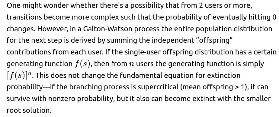
When we have more than 1 user, each user can individually produce 0, 1, or 2 "successor" users according to the same distribution. Hence the total user count next day is the sum of independent identically distributed random variables (one for each current user). The question is: starting from 1 user, what is the probability that eventually the entire process will go extinct (meaning the app hits 0 users at some point in the future)?
Galton-Watson Process Setup
The probability generating function (PGF) of the number of new users contributed by a single existing user is
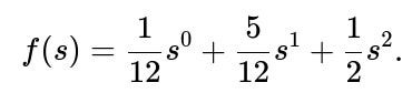

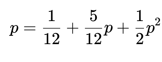
Let p be the extinction probability starting from 1 user. We know from branching process theory that p satisfies the fixed-point equation
p=f(p),
where f(⋅) is the probability generating function for a single “parent” user. Substituting the values:
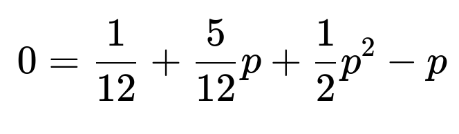
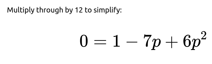
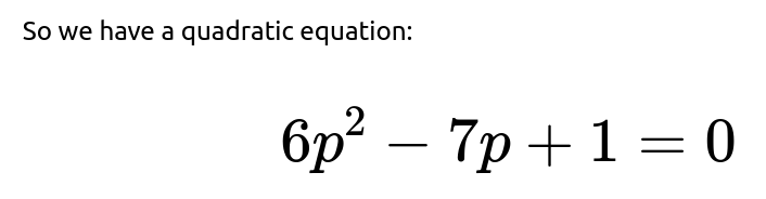
We can rearrange and solve for p. Move all terms to one side:
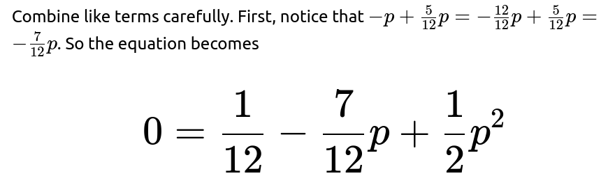
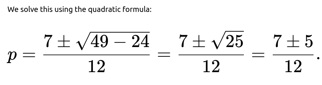
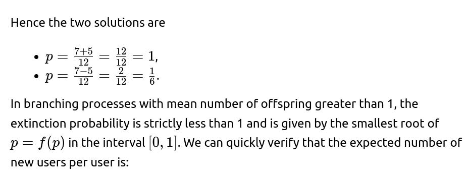

Because the mean is indeed greater than 1, the correct extinction probability is the smaller root. Therefore, the probability that the app eventually hits 0 users, starting from a single user, is:
Thus, the short answer to the original question is that the probability the app eventually hits 0 users is 1/6.
Implementation Example in Python
Below is a small Python snippet demonstrating how one could solve that quadratic equation programmatically. Although it is straightforward, it shows how to verify the extinction probability numerically:
import math

# Coefficients for 6p^2 - 7p + 1 = 0
a = 6
b = -7
c = 1

discriminant = b**2 - 4*a*c
root1 = (-b + math.sqrt(discriminant)) / (2*a)
root2 = (-b - math.sqrt(discriminant)) / (2*a)

# Typically for supercritical branching processes, extinction prob is the smaller root in [0, 1]
extinction_prob = min(root1, root2)
print(extinction_prob)  # Expected to be 1/6
This script should print out 0.166666..., which is indeed 1/6.
Subtle Points and Edge Cases
Another subtlety is that p=1 is always a solution to p=f(p) for any branching process because if we assume the population definitely goes extinct, that is a trivial fixed point of the generating function. However, the physically meaningful answer in a supercritical regime is the smaller of the two roots in [0,1], which is 1/6 in this problem.
Finally, we assume that day-to-day transitions happen independently and identically according to the stated probabilities. If real-world effects (e.g., correlation of user decisions, external advertising, saturating user interest) come into play, the model might change, but for the puzzle’s scope, the standard branching process approach addresses the question thoroughly.
How would you explain this solution if the interviewer wanted you to justify using a branching process framework?
A branching process is a natural way to model phenomena where each “entity” (in this case, a user) can give rise to some random number of new entities (other users), and we track the total population across discrete time steps. The essential assumptions are:
Each user acts independently in terms of whether they stay, leave, or cause new users to join.
The probability distribution governing these new users is the same for all current users (i.i.d. offspring counts).
Given those assumptions, the standard extinction probability derivation for Galton-Watson processes applies, which tells us to look for solutions to p=f(p), where f(s) is the generating function of the offspring distribution. This approach provides a closed-form solution for the probability that the process eventually dies out. Hence, modeling the app’s user count as a branching process is justified by the problem statement’s suggestion that each user on a given day can independently yield 0, 1, or 2 users the next day with given probabilities.
What if the interviewer asked about the average time to extinction or whether the app might blow up in user count?
Beyond the extinction probability, we might consider:
The expected time to extinction: In a branching process, the mean time to extinction can be infinite if the process is supercritical and the extinction probability is less than 1. Since our mean is 17/12>1, there's a nonzero probability the app lives forever. Conditional on eventual extinction, you can compute expected time to extinction, but the unconditional time might be infinite due to the positive chance of indefinite survival.
The chance of “blowing up” in user count: This is simply the complement of extinction probability, which in this case is 5/6. That 5/6 figure is the probability that the app’s user count never returns to zero and presumably “survives” indefinitely in the idealized model.
Suppose the interviewer follows up by asking how the answer changes if the expected number of new users per user was less than or equal to 1?
If the expected offspring (new users per existing user) is ≤1, the process is said to be critical (=1) or subcritical (<1). In both cases, for a Galton-Watson process, the extinction probability equals 1. Specifically:
In the critical case, E[offspring]=1, and the process will almost surely die out eventually. It might fluctuate for some time, but eventually it hits 0 with probability 1.
In the subcritical case, E[offspring]<1, and the population shrinks on average, so again the process goes extinct with probability 1.
In the problem at hand, the expected number is 17/12>1, so it is a supercritical case. That’s why the extinction probability is less than 1 (namely 1/6).
How would you double-check the correctness of your result during an interview if you can't rely solely on memory of branching processes?
You can verify correctness in several ways:
Numerical simulation: Write a simulation that simulates many realizations of the process from 1 user, tracking whether it eventually hits 0. After many trials, the fraction of trials that go extinct should be close to the analytical result (1/6). This simulation-based approach is a powerful demonstration in an interview.
Checking boundary conditions: If we artificially changed probabilities (e.g., made it certain that from 1 user we always spawn 2), we know the chance of extinction should be 0, because it grows exponentially. On the other hand, if the probability of going to 0 was very high and dominating, we’d expect the app to always eventually die out. The final answer of 1/6 lies reasonably in between.
Analytical reasoning consistency: The derivation that the extinction probability solves the equation p=f(p) is standard branching process theory, so if the arithmetic is consistent and the expected number of offspring is indeed above 1, the smaller root is the correct physical solution.
All these points cross-validate the correctness of 1/6 as the extinction probability.
Could there be a tricky follow-up where the interviewer suggests that once the user base reaches a certain threshold, other factors come into play?
Yes. In real-world scenarios, user growth may not remain governed by the same probabilities once the user base is large. For instance:
Network effects could make it more likely for more users to join as the user base grows (changing the distribution and potentially reducing the chance of extinction further).
Saturation effects or limited market size might reduce the growth probability over time.
Changes in user behavior, app updates, or external influences might invalidate the i.i.d. assumption.
However, for the puzzle-like question asked in the interview, we treat the transition probabilities as uniform and unchanging for all time. The final answer remains 1/6 unless we alter those assumptions.
If the interviewer asked for code to perform a Monte Carlo simulation to estimate the probability of extinction, how could you illustrate it?
Below is a simple Python sketch for a Monte Carlo simulation of the described branching process. It’s purely for verification and demonstration.
import random
import statistics

def simulate_branching_process(num_simulations=100000):
    extinctions = 0
    for _ in range(num_simulations):
        # Start with 1 user
        current_users = 1
        while current_users > 0:
            next_users = 0
            # Each user can go to 0, 1, or 2 independently
            for _ in range(current_users):
                r = random.random()
                if r < 1/12:
                    # 0 new
                    next_users += 0
                elif r < 1/12 + 5/12:
                    # 1 new
                    next_users += 1
                else:
                    # 2 new
                    next_users += 2
            current_users = next_users
            # If it eventually hits 0, break out
            if current_users == 0:
                extinctions += 1
                break

    return extinctions / num_simulations

prob_est = simulate_branching_process()
print("Estimated extinction probability:", prob_est)
This code initializes a single user, evolves the process day by day, and tracks whether it hits zero. Repeat that for many simulations. Over enough runs, the empirical estimate for the extinction probability will hover around 1/6.
Below are additional follow-up questions
If the process is time-varying, how does that affect the probability of eventually hitting zero?
When the transition probabilities or offspring distribution can change over time, the standard Galton-Watson framework with a single, constant probability generating function no longer strictly applies. Instead, you might have a branching process in which each generation has its own probability generating function depending on the time step. In such a case, the probability of extinction may be analyzed by composing different generating functions across each day. Specifically, if you denote the generating function at day ( t ) as ( f_t(s) ), then the overall population evolves by applying ( f_1(s), f_2(s), \dots ) sequentially. The event of eventual extinction depends on whether these time-varying offspring distributions collectively still allow a surviving lineage with nonzero probability.
A practical approach is:
Write out the day-by-day distribution of new users per current user. For day 1, each user contributes 0/1/2 users with some probabilities; for day 2, each user might have a different probability distribution, and so on.
The extinction probability may be bounded or computed by repeatedly iterating each day’s generating function on an initial guess (like ( s=0 ) or ( s=1 )). This can get complicated because you might lose the simplicity of a single fixed-point equation ( p = f(p) ).
Monte Carlo simulation can be particularly valuable. You simulate the daily transitions with the correct day-specific distribution many times and estimate how often the process hits zero.
A subtle pitfall is that if the expected offspring distribution remains above 1 at some time steps but dips below 1 at others, you may have intervals of fast growth followed by intervals of contraction. Ensuring the entire population goes extinct (or survives) might hinge on delicate day-by-day dynamics. Depending on real-world considerations (e.g., marketing campaigns on specific days or seasons), the user population trajectory may vary drastically.
What if users' decisions are correlated rather than independent?
The classic Galton-Watson theory relies on the assumption that each user’s behavior—staying, leaving, or recruiting new users—is independent of others, given the current population. Realistically, users’ decisions can be correlated. For instance, if a user sees many friends leaving, they might also be more likely to leave. If the user sees many friends staying active, they might recruit additional friends. In such correlated scenarios, the distribution of the number of “new” users each day is not simply the product of identical independent trials.
To handle correlation, you might instead view the system as a Markov chain in which the state is the entire user population size (or even more detailed user attributes). For each state ( n ), you have a probability distribution for transitioning to some new state ( m ). If user decisions are correlated, deriving a simple probability generating function for “one user’s offspring” no longer holds. Instead, you would specify a transition matrix ( P ) where ( P_{n,m} ) gives the probability of moving from ( n ) users to ( m ) users in one day.
Even with Markov chains, the extinction probability still equates to the probability that the chain eventually hits the state 0. However, computing that might require analyzing absorbing Markov chains or performing a more advanced state-based analysis. A potential pitfall is that if correlation strongly promotes mass exodus (i.e., once some users leave, many others follow), the chance of extinction can be higher than predicted by an independent-user model. Conversely, if correlation promotes retention (a viral growth effect), extinction might become much less likely.
Could the process ever spontaneously recover from zero users?
In the original setting, once you hit zero, you remain there (because no users exist to recruit new ones). But in real-world scenarios, an app can sometimes re-emerge from zero if an external factor injects new users. That changes the question from “what is the probability of hitting zero at least once?” to “what is the probability of hitting zero and staying there without new external stimuli?”
If spontaneous re-entry is possible, then zero is no longer an absorbing state. Your Markov chain or branching-process-like model would have transitions from 0 users to some positive number of users with some probability (which might represent external marketing or random new sign-ups). In that case, you can’t talk about a strict extinction probability in the classical sense, because the system can keep leaving zero. You might then be interested in the probability of hitting zero at any point in time, or how often the chain stays near zero for a prolonged period. A practical pitfall is ignoring external re-injection of users, especially if the app invests heavily in marketing whenever the user base starts to plummet.
How do results change if each user can bring in more than 2 new users with some probability?
In the original problem, each existing user has a probability distribution over 0, 1, or 2 new users. You can generalize this to any distribution over ( k \ge 0 ). For instance, you might have:
Probability ( p_0 ) of 0 new users
Probability ( p_1 ) of 1 new user
…
Probability ( p_n ) of ( n ) new users with ( \sum_{k=0}^{\infty} p_k = 1 ).
The probability generating function would then be [ \huge f(s) = \sum_{k=0}^{\infty} p_k s^k. ] The extinction probability ( p ) still satisfies [ \huge p = f(p). ] You solve for the smallest nonnegative root of that equation in ([0,1]). The main pitfall is ensuring the solution remains in the valid range [0,1] and interpreting which root is physically meaningful. If the expected number of offspring is greater than 1, the process is supercritical and there is a smaller root in (0,1). If it equals 1 (critical), the extinction probability is 1. If it is less than 1 (subcritical), extinction is also 1.
When the maximum number of offspring is greater than 2, the user population might explode more rapidly in some scenarios, further lowering the extinction probability. However, if the distribution remains such that the mean is still below or equal to 1, extinction will remain guaranteed.
What if we only care about hitting zero within a finite number of days?
Sometimes, the question might not be about “eventual” extinction but rather about the probability that the process hits zero on or before some deadline ( T ). For example, maybe the investor wants to know the chance that the user base collapses within one year. That question is different from “ever hitting zero in the infinite horizon.”
In a Markov chain viewpoint, you can compute the probability of being in state 0 at or before step ( T ) by summing up all paths that lead to 0 by time ( T ). Alternatively, you can simulate or recursively calculate: [ \huge P(\text{hit } 0 \text{ by time } T) = P(\text{hit } 0 \text{ by time } T-1) + P(\text{not hit } 0 \text{ by time } T-1) \times P(\text{transition to 0 at time } T). ] In branching processes, you typically track the distribution of population size at each generation. One pitfall is that “eventually hitting zero in infinite time” might be quite different from “hitting zero by day 10,” particularly in a supercritical regime where large expansions can happen quickly. If that expansion occurs, the short-term probability of hitting zero might actually be small, even though in the infinite horizon there is still some extinction probability.
What if the process starts with more than one user and the user addition probabilities differ for the first user vs. subsequent users?
Sometimes, an app’s first user is “special” (like a founder or a power user) who might have different odds of attracting new users than a typical user. This breaks the i.i.d. assumption at the heart of a standard Galton-Watson model. The process might be described by a multi-type branching process where “type A” user is the founder who has one distribution of offspring, while “type B” users have a different distribution. The extinction probability then depends on the interplay between these user types.
You might define two generating functions ( f_A(s) ) and ( f_B(s) ) and track how each type replicates into further types. The extinction criterion becomes the condition that all lineages from both types eventually vanish. A notable pitfall is incorrectly aggregating the reproduction rates across different user categories. If you just combine them incorrectly into a single distribution, you might misestimate the extinction probability. In practice, a multi-type approach keeps track of a vector of generating functions.
How does user churn factor in if it depends on how many days a user has already stayed?
Realistically, the probability a user leaves might increase or decrease the longer they have been on the platform. A newly onboarded user might be more likely to churn quickly, or conversely, they might be more excited and remain for a while. This leads to an age-dependent or state-dependent process, where each user’s churn and recruitment probability depends on their “age” or “cohort.”
In a basic Galton-Watson process, every user is considered identical each day, and their probability distribution for creating new users is identical and memoryless. But if churn depends on age, the process no longer has the same identical distribution for each user. You might need to employ more general age-dependent branching processes (sometimes known as Sevast’yanov processes), or a sophisticated Markov chain with expanded state representation that includes the user’s age or membership cohort. Calculating extinction probabilities in such age-dependent models can be more intricate. The main pitfall is oversimplifying by ignoring user tenure and how it might affect churn or recruitment.
Could cyclical user behavior (e.g., weekly cycles) cause repeated near-zero dips that might still not constitute true extinction?
In some apps, user engagement might ebb and flow in predictable cycles—like dropping on weekends and picking up on weekdays. This can create cyclical patterns in user counts, and it is conceivable the user base could get very low on certain days yet rebound on others. To truly hit zero, it must be that on a given day, nobody logs in or continues using the app. Cyclic behavior complicates the analysis because a near-zero dip on a slow day might not guarantee the process is close to extinction if a strong rebound is likely on the following day.
In a Markov chain formulation with daily or weekly transitions, you might see a state space that interprets “Monday’s user base” separately from “Tuesday’s user base,” or you might treat each day as a single step but incorporate day-specific transition rules. You could have a cyclical chain of transition matrices ( P_1, P_2, \ldots, P_7, P_1, P_2, \dots ) repeating for each day of the week. The pitfall is mistakenly using a single matrix to describe daily transitions if the transitions truly vary across days.
What if we want to estimate confidence intervals around the extinction probability rather than just a point estimate?
Analytically, for a simple Galton-Watson process with a known offspring distribution, you can solve for the extinction probability exactly. In real-world scenarios, the probabilities themselves might be estimated from data, meaning there is statistical uncertainty in the parameters. If you want to give a range (confidence interval) for the extinction probability, you need to:
Estimate the distribution parameters from empirical data.
Perform a statistical procedure (like a bootstrap) that repeatedly resamples from your data to produce different plausible estimates of the user transition probabilities.
Solve for the extinction probability under each set of estimated parameters.
Take a percentile range of these estimates as your confidence interval.
A typical pitfall is to report a single extinction probability from a point estimate of the transition probabilities without reflecting uncertainty in the data. If your sample data is small or has sampling bias, the actual extinction probability might differ from your best guess. Reporting intervals or robust estimates helps handle real-world variability.
How do you handle continuous-time models where user arrival and departure can happen at random intervals?
The given puzzle is a discrete-time daily process, but in many apps, user actions can happen at any time. A continuous-time branching process (like a birth–death process) can model the user count’s random trajectory. Instead of day-by-day transitions, you track rates of new user arrivals and departure events in continuous time. You might specify:
A birth rate (\lambda) for each current user, meaning each user independently spawns new users at some rate.
A death rate (\mu) for each current user, meaning each user independently churns at some rate.
From those rates, one can compute the probability of eventual extinction in a continuous-time Galton-Watson or birth–death setting. A pitfall: if your data or domain is truly continuous, forcing a daily-step model may hide important details (like multiple join/leave events within a single day). On the other hand, modeling continuous time can be more mathematically complex. Whether you choose discrete or continuous time often depends on how your data is collected and what your assumptions about user behavior are.
How would you factor in marketing interventions that occur if the user base starts to decline?
In real practice, an app owner might launch an intervention whenever the user base is observed to decrease below a certain threshold. This intervention could push the user base back up. Such interventions break the straightforward branching process assumption, because the probability distribution changes conditionally on the event that user numbers are low.
One approach is to define a piecewise Markov chain or a “threshold-based” policy model:
If the user count is above threshold ( h ), normal transition probabilities apply.
If the user count falls at or below ( h ), a marketing push changes the transition probabilities, giving a higher probability of new sign-ups.
In terms of extinction, you might have a “soft floor” at that threshold if marketing is strong enough, meaning true extinction could become much less likely or even impossible if these interventions guarantee that once the user base drops, new users are always pulled in. A pitfall is ignoring such real-world strategies and erroneously concluding the app might have a certain extinction probability. In reality, the marketing intervention could drastically reduce that probability.
What differences arise if the state space has an upper bound on the number of users?
Real platforms often have practical or effective upper limits—servers can only handle so many users, or there’s a limited target population. In a branching process, we often assume population growth can continue indefinitely, but physically or socially, it can saturate. If we cap the number of users at some ( M ), then the chain is finite-state with a maximum population. In a finite-state Markov chain, you either have:
0 as an absorbing state if re-entry from 0 is impossible.
Possibly an absorbing state at ( M ) if once the user base is full, it cannot grow further.
The extinction probability then depends on whether state 0 is reachable from states near ( M ). You analyze transition probabilities in a finite Markov chain and can compute exactly the probability of eventually being absorbed in 0 (extinction) or in ( M ) (full saturation). A subtle pitfall is ignoring that saturations can happen in real life: maybe the network effect saturates at some limit but churn continues to be nonzero, so the chain can bounce around near the top. Whether 0 remains absorbing depends on whether spontaneous new sign-ups from outside are allowed or not.
In practice, how might you validate that this branching process model is a good fit for the social media app?
To validate the model, you would gather data on day-to-day user transitions—i.e., how many new users appear for each current user. You would check whether:
Each user acts independently in recruiting new users or leaving.
The probabilities remain stable over time (stationarity).
The daily transitions do indeed match the distribution used.
Empirically, you might build a histogram or distribution of how many new users each existing user “brings” from one day to the next. If that distribution matches your model (like 1/12 chance of 0, 5/12 chance of 1, 1/2 chance of 2), then a Galton-Watson process with that distribution is plausible. Another step might be to measure correlation. If you observe that when one user leaves, others are more likely to leave, that signals correlation that the standard branching model doesn’t capture.
A major pitfall is blindly applying the branching process formula for extinction probability if real data contradicts the independence or stationarity assumptions. In that case, your computed value (like 1/6) might be far off from observed behavior.