
ML Interview Q Series: Predicting App Extinction Probability Using Branching Processes and Generating Functions.

Browse all the Probability Interview Questions here.
11. You are analyzing the probability of failure or success of a small social media app competitor. Using some initial data, you estimate that if there is 1 user, after a day there is a 1/12 chance of having 0 users, 5/12 chance of staying at 1 user, and 1/2 chance of going to 2 users. If the app starts with 1 user on day 1, what is the probability that the app will eventually have no users?
Understanding this problem can be approached through the lens of a Galton–Watson branching process or, more simply, through the concept of a discrete-time Markov chain with probabilities of transitioning between states of “number of users.” The key insight is that if each current user “generates” a certain random number of users in the next day (with known probabilities), we can use the probability generating function to find the probability of ultimate extinction (i.e., eventually reaching zero users).
The essential facts given are: There is exactly 1 user at day 1. After a single day (from exactly 1 user), the probabilities of next-day outcomes are: 1/12 chance of going to 0 users 5/12 chance of staying at 1 user 1/2 chance of going to 2 users
We want the probability that eventually, after some finite (but possibly random) number of days, the user count goes to 0.

We define the generating function
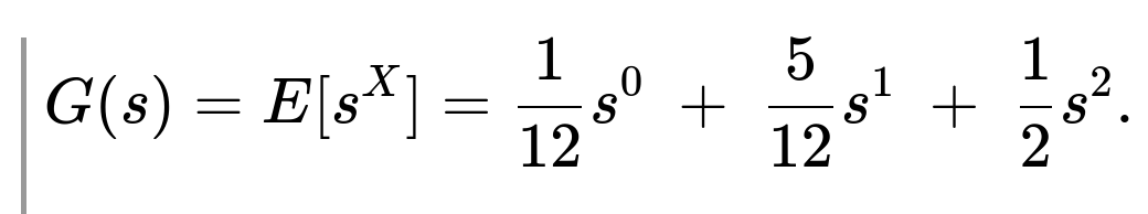

In the theory of branching processes, the probability q of eventual extinction (i.e., ultimately reaching zero users at some time in the future) is the smallest nonnegative solution to the equation


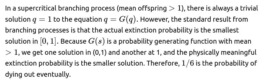
For a branching process with mean offspring >1 (which is called supercritical), the probability of extinction is strictly less than 1, and we must pick the unique solution in [0,1] that is less than 1. We observe that the mean number of new users from one current user is:
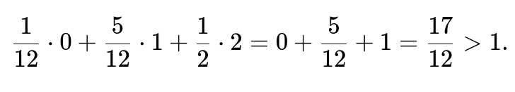
So, this process is supercritical, which means it has a nonzero probability of never reaching zero users. Therefore, the probability of eventually reaching zero is not 1 but rather the smaller root of the generating function equation, which is 1/6.
Thus, the probability that the app will eventually have no users, starting with 1 user, is 1/6.
A Python snippet to quickly verify the smaller solution:
import sympy as sp

q = sp.Symbol('q', real=True)
expr = 6*q**2 - 7*q + 1  # 6q^2 - 7q + 1 = 0
solutions = sp.solve(expr, q)
print(solutions)  # Should see [1/6, 1]
Running this will show the two solutions, 1 and 1/6, confirming that 1/6 is the extinction probability.
Explaining Why We Select 1/6 as the Extinction Probability
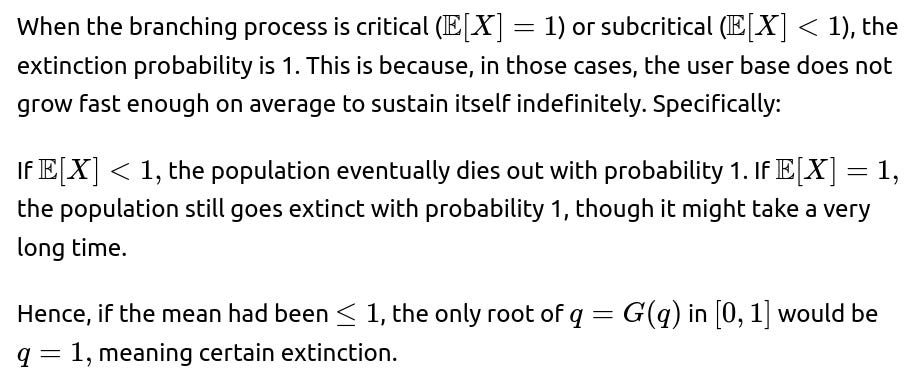
We know from branching process theory that if the expected offspring number (the expected number of next-day users per current user) is greater than 1, there is a nontrivial chance that the population (user base) survives indefinitely. The extinction probability in such a scenario is the smaller real root of q=G(q). If the mean were less than or equal to 1, the extinction probability would be 1 (or the only solution). Since our mean here is 17/12, the smaller root is strictly less than 1, so 1/6 is the correct extinction probability.
Additional Technical Insight on the Generating Function Approach
When dealing with a random process where each user can “branch” into a stochastic number of new users on the next day, we can treat each user’s behavior as an independent trial. The key result is that the total probability of extinction (having no users eventually) is the unique fixed point of the generating function G(s) in the interval [0,1], provided the mean offspring count is greater than 1. This stems from the fixed-point theorem in branching processes.
Insights for Real-World or Interview Follow-Up Queries
It may be asked why the solution is not 1. After all, the probability of going from 1 user to 0 users in a single day is 1/12, so how come we do not sum up probabilities over multiple days? The short explanation is that even though on any given day there is a chance to drop from 1 user to 0, there is also a significant chance to grow in user count, which can sustain the population for a much longer period or indefinitely. Summing infinite paths in a naive way is not correct; instead, we rely on the standard branching process result and solve for the extinction probability via the generating function.
Below are potential follow-up questions and highly detailed answers that a FANG-level interviewer might ask to probe deeper into your understanding.
What if the expected value of new users from a single user were less than or equal to 1? Would that change the extinction probability?
Could you interpret the probability of eventually reaching 0 in terms of a Markov chain perspective rather than a branching process?
Yes, we can. We can regard the number of users as a Markov chain on the nonnegative integers, where from state 1 we have transitions:
1 → 0 with probability 1/12 1 → 1 with probability 5/12 1 → 2 with probability 1/2
Then we would need transitions from 2 users, 3 users, etc., to analyze the chain’s behavior in full. In a standard Galton–Watson setting, each user acts independently and “spawns” some distribution of new users, which leads to a well-known probability generating function approach. But from a Markov chain perspective, you would formalize transition probabilities from every state nn to other states. Under the independence assumptions of a branching process, that chain has a structure that can be fully captured by the same generating function argument.
Why do we discard the root q=1 and select q=1/6 as the extinction probability?
How can we intuitively check that 1/6 makes sense?
We know that each day, from a single user: There is a non-trivial chance (1/2) to double the user base, which can spur exponential-like growth. At the same time, there is only a small chance (1/12) to drop to zero users immediately. Over many days, if the community can keep doubling quickly enough, there is a significant chance to keep growing. Nevertheless, there is still a possibility that random fluctuations cause the community to fail. Numerically, it turns out that possibility is 1/6 in the long run.
Could you give another quick example of finding the extinction probability via generating functions?

or some expression that in the correct domain lies in (0,1). (One would solve for q in the same way as in the original example.)
This is just to show how the same formulaic technique applies to many branching distributions.
Are there any assumptions we implicitly used that might be violated in real-world social media app growth?
Independence of user decisions day to day: We assumed each current user acts independently in whether or not they attract or lose users. Real apps have network effects that can introduce correlation between user behaviors. Homogeneity: We assumed the transition probabilities are stationary (they do not change over time). In practice, user acquisition or churn can change drastically over time if new features are introduced or marketing changes. Discrete-time updates: We treat user changes as happening in a single daily step. Actual processes might be continuous or have more frequent updates. No “carrying capacity” or upper limit: The branching process does not incorporate an upper bound. Real social media growth might saturate or have competition constraints.
These factors can complicate real-life prediction and might mean the 1/6 figure is only an approximation for the probability of eventual app failure if the environment remains static and user growth follows the same distribution.
Could we approximate the solution numerically if we forgot the generating function approach?
Yes. One might attempt to do a stochastic simulation. For instance, you can write a Python simulation that starts with 1 user, and at each step draws a random next-day count from the given distribution for each user (or from some Markov chain logic). Repeat the simulation many times (Monte Carlo) and estimate the fraction of runs that eventually drop to zero. With enough samples, you will empirically approach the correct extinction probability. However, the generating function approach is exact.
Below is a basic illustrative Python simulation. This is not a perfect real-world model but demonstrates how one might approximate the extinction probability.
import random
import statistics

def simulate_one_run(max_days=10000):
    # Start with 1 user
    users = 1
    for day in range(max_days):
        new_users = 0
        # For each user, pick next-day count. In a simpler approach, we assume
        # the entire population transitions according to the distribution, as given.
        # For a branching process, you'd sample for each user individually.
        # But here let's do a direct single sample from the distribution for the entire population
        # if there's exactly 1 user. If there's more, you would define transitions from those states.
        # A more accurate approach for pure branching:
        #   new_users = sum(single_draw for each user in range(users))
        # For the question's distribution from 1 user:
        #   we only have that distribution from a single user scenario.
        # So let's keep it simpler and just use the known distribution from 1 user for demonstration.
        if users == 1:
            r = random.random()
            if r < 1/12:
                users = 0
            elif r < 1/12 + 5/12:
                users = 1
            else:
                users = 2
        else:
            # This is incomplete because we don't have the distribution from 2 or more users in the question.
            # We'll just do a naive assumption for demonstration:
            # For each of the 'users' individuals, sample from the same distribution
            # so new_users = sum of individual user expansions.
            for _ in range(users):
                r = random.random()
                if r < 1/12:
                    # This 1 user disappears
                    new_users += 0
                elif r < 1/12 + 5/12:
                    new_users += 1
                else:
                    new_users += 2
            users = new_users

        if users == 0:
            return True  # extinct
    # If we didn't hit 0 within max_days, treat as survived
    return False

num_simulations = 100000
extinct_count = 0
for _ in range(num_simulations):
    if simulate_one_run():
        extinct_count += 1

estimated_probability = extinct_count / num_simulations
print("Estimated extinction probability:", estimated_probability)
The above is a rough illustration. In a more careful approach for a pure branching process, you would do exactly the sum-of-independent draws for each user. The result from such a simulation would converge, for large runs, to around 1/6. However, the code above tries to handle transitions from 2 or more users by reusing the same distribution for each individual user, which is more consistent with a branching process. If that distribution truly applies identically and independently for each user, the average result converges to the same theoretical 1/6 in the large limit.
How does knowing the extinction probability help in real business decisions?
It gives a sense of the “risk of total failure” under a simplified model of user growth. If that risk is high, you might adopt strategies that increase user retention or accelerate user acquisition so the effective number of new users per current user goes up. If you push the mean number of new users per user far enough above 1, your extinction probability can shrink even further.
That said, real ecosystems are much more complex than a simple branching/Markov model. Still, this line of reasoning is valuable as a conceptual tool to clarify how a small difference in average growth above or below 1 can drastically change long-term outcomes.
Having walked through each subtlety, the definitive short answer is that the probability of eventually reaching zero users is the smaller solution to the generating function fixed-point equation. That solution is 1/6.
Below are additional follow-up questions
What if the transition probabilities are not fixed but change over time?
Changing transition probabilities over time means that each day’s probability of going from 1 user to 0, 1, or 2 users might depend on external factors (e.g., marketing campaigns, seasonal trends). In a Markov chain context, this would no longer be a time-homogeneous chain. Likewise, in a branching process framework, the “offspring distribution” could vary by generation.
One immediate consequence is that the standard probability generating function technique, which relies on a stationary offspring distribution (the same distribution for each day or generation), no longer directly applies. Instead, one might construct a time-inhomogeneous branching process or Markov chain. The eventual extinction probability can sometimes still be computed via iterative methods, but you lose the simplicity of a single fixed-point equation.
A practical approach is to break time into distinct periods (e.g., day 1–10, day 11–20, etc.), estimate the distribution for each period, and then iteratively calculate the extinction probability by conditioning on each period’s potential transitions. For instance, you might do this step by step:
Define the extinction probability after day 1 as a certain function of day-1 transition probabilities.
Move to day 2 with new probabilities, incorporate them into your analysis, and propagate forward.
You might use dynamic programming to track P(extinction∣initial number of users=n) across each day. The key pitfall is that if transition probabilities become more favorable in the future (e.g., bigger marketing pushes), the extinction probability might decrease significantly compared to a stationary model. Conversely, if user acquisition probabilities worsen (e.g., competition intensifies), extinction probability could be higher.
In real-world scenarios, ignoring time-varying effects can drastically misestimate the actual risk of failure. If you incorrectly assume stationarity when in fact the process evolves (e.g., you suddenly see a spike in user interest from a viral ad campaign), your model could show a gloomier or rosier picture than the reality.
How do we handle the situation where the number of new users could be larger than 2 in a single day?
In the question’s simplified distribution, each day from a single user you only go to 0, 1, or 2 users. Realistically, one user might invite many more than 2 new users in a short time (e.g., viral growth). If we allow for a random variable X that can take values 0, 1, 2, ..., up to some potentially large integer, then the generating function becomes:


One pitfall: if you try to handle an unbounded distribution, the equation may not be a simple quadratic or cubic—it can be more complicated, potentially requiring numerical methods (like iterative root-finding) to identify the solution in [0,1]. Another pitfall is data scarcity: real growth might have a “fat tail” (small probability of extremely large new user influx), which can disproportionately affect the extinction probability.
How might we model partial user “inactivity” or churn rather than a hard drop to zero users?
The question’s transitions revolve around going from 1 to 0, 1, or 2. But real apps can have users remain nominally registered while becoming partially inactive. Churn might be a gradual process, with some fraction of active users dropping off. One way to incorporate partial activity into a branching process is to expand the state space:
• “Active” users. • “Inactive” users (possibly reactivatable). • “Completely gone” users (cannot return).
You might build a multi-type branching process in which each active user transitions to a certain distribution of active/inactive users next day. Inactive users might have a certain probability to return to active or go to “gone.” This multi-type approach leads to a higher-dimensional generating function. In matrix form, you track probabilities of transitions among types. The extinction probability is now the probability that the number of active users goes to zero (even if some are still “registered but inactive”).
A major pitfall is complexity: multi-type branching processes require a matrix-based approach or vector generating functions. The simpler approach is to treat all non-active (including unsubscribed) as “zero users,” but that can severely overestimate extinction if many users are just temporarily inactive.
How do you incorporate the idea that once the user base is large, it might be harder to lose everyone?
In real-world scenarios, a large user base can develop self-sustaining network effects. The chance of dropping from a large user base directly to zero in a short time can be extremely small (though still possible over the long run). A naive branching model might not reflect “stabilizing” forces when the user base grows. One might incorporate such stabilizing forces by capping the downward transitions: for instance, from n users, the distribution heavily favors staying at high user counts. Alternatively, you could impose a logistic or saturating growth function.
From the Markov chain perspective, states representing large user counts might have an extremely small probability of going to near zero in a single step. A more realistic approach is to define a transition distribution that depends on n, not just on single-user behavior. If you truly believed each user acts independently, the branching process approach might still hold, but real network effects often reduce churn as the user base grows.
One pitfall is ignoring the path dependency: if you have a big user base, small fluctuations are less likely to kill the system outright, but catastrophic events (e.g., scandal, data breach) might cause a huge exodus of users. Thus, advanced models might incorporate “shock events” that are improbable but can cause massive churn. Such events rarely appear in simple branching models, so ignoring them can give overly optimistic survival probabilities.
What about the time it takes to either go extinct or grow? Is there a way to estimate the expected time to extinction?
Yes. The same theory that gives the extinction probability can often be extended to estimate the distribution of extinction times. For simple offspring distributions, you might attempt an explicit formula or use iterative or simulation-based methods.
A typical approach uses:

An alternative approach is to rely on well-known results for Galton–Watson processes, which sometimes give closed-form or at least series expansions for the expected time to extinction:
Pitfalls and edge cases:
In supercritical cases, you can have infinite expected survival time for the entire process if there’s a chance it explodes. Yet among the lines that do die out, you can estimate how many days (on average) it takes.
In practice, you may not only be interested in the average time to extinction but also the distribution’s tail—rare scenarios in which the system lingers with a small user base for a very long time before vanishing.
Could certain non-branching-process approaches (e.g., differential equations) approximate this problem?
Sometimes, especially for large user populations, people use ordinary differential equations (ODEs) or difference equations to approximate expected user growth:
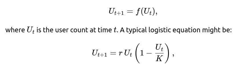
where r is a growth rate and K is a carrying capacity. This is a purely deterministic approach that models expected behavior but does not incorporate stochastic extinction in the same manner. The big difference from branching processes:

In real interview scenarios, you might mention that ODE or difference equation methods can be helpful to analyze average growth trends, but for extinction or total failure probabilities, a discrete stochastic approach (branching process, Markov chain, or Monte Carlo simulation) is generally more appropriate.
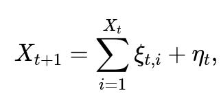
What if an external investor injects new users periodically, effectively “rescuing” the app from extinction?
An external agent periodically boosting user count changes the dynamic. For instance, suppose every Monday, a marketing campaign ensures 10 new signups. This is akin to having a “forced immigration” of new individuals into a population, making pure extinction impossible unless the immigration stops. Some branching process models include immigration:
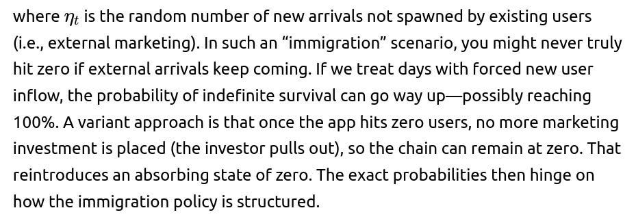
Pitfalls:
• Overly optimistic calculations that ignore the possibility that the external sponsor stops injecting users if usage is too low. • Underestimating the random timing. If the app hits zero before a scheduled injection, it might be “officially” considered dead or removed from the market.
If the extinction event happens, how might we measure partial “revival” scenarios?
In the usual branching process or Markov chain model, state 0 (no users) is an absorbing state: once the system has no users, it stays at zero forever. But in reality, an app could have 0 daily active users today, then some new user could appear tomorrow by stumbling on the app. This breaks the assumption that zero is truly absorbing. So a refined model can include a small probability of spontaneously “reappearing,” effectively a transition 0 → 1 with some probability if the app is still accessible.
The main difference:
• If 0 is not truly absorbing, the concept of “extinction probability” might shift to “probability of eventually returning to nonzero.” • The chain might wander in and out of the zero state.
Pitfalls:
• Overcounting indefinite revivals if the probability from 0 to 1 is non-negligible. You might end up with zero not being a stable or absorbing state, so standard extinction formulas for branching processes no longer apply straightforwardly. • Realistically, once an app has 0 active users, it might remain in a dormant state from which it can only be revived by external marketing. So again, you’d need to incorporate that “rescue” or “random discovery” mechanism.
How could domain-specific constraints, like app store removal, alter the probability of extinction?

Pitfalls:
• Overly simplistic threshold rules can skip the possibility that the user count might bounce back just before dropping below T. Real policy might look at usage for consecutive months or have a grace period. • If the threshold is high, the chance of eventually dropping below it might be significantly different from the chance of literally hitting zero.
Could partial success states matter, even if the user count never truly hits zero?
In some business contexts, “extinction” means not necessarily zero users, but dropping below a certain viability level, such as being unprofitable or no longer able to pay infrastructure costs. For example, if you need at least 10,000 daily active users to break even, dropping below that for multiple days might effectively be “extinction” from a business standpoint—even if you still have 5,000 loyal users. That can be treated like the threshold scenario. You then model absorbing states that reflect an unviable user base. The classical branching or Markov approach can still be adapted: define any state below 10,000 as an effective “sink.” The probability that you eventually enter that sink is your “extinction” risk from a profitability perspective.
Pitfalls:
• The threshold might be dynamic (for instance, as infrastructure costs grow or shrink, the break-even point changes). • Real businesses might pivot, further complicating the assumption that dropping below 10,000 daily users means guaranteed closure.
Is there a possibility of cyclical fluctuations in user count, and how would that affect eventual extinction?
Yes, user counts might fluctuate seasonally or with viral cycles. In a simpler Markov or branching setting, we assume no cyclical changes beyond random daily draws. In reality, you can have weekly or monthly cycles (e.g., usage is high on weekends and lower on weekdays). Over many cycles, the user base might slowly drift up or down. Even if the average is above 1 user per user per cycle, daily or weekly dips might threaten extinction in the early phase when the base is small.
A thorough analysis could embed a cyclical factor in the model:

Over each cycle, compute net growth or decline.
If the average over the entire cycle is still above 1, you might remain supercritical in a cyclical sense, meaning a non-zero chance of indefinite growth. However, short extreme dips in the cycle could cause the user base to go to zero if it is small enough during that dip. This interplay can make the extinction probability higher than an “average-based” stationary model would predict.
Pitfalls:
• Failing to account for the fact that cyclical extremes can kill a small base more easily. • Overcomplicating the model if the cyclical effect is minor compared to the overall average. In an interview, emphasize that you’d evaluate the relative magnitude of the cycle compared to the drift.
What if some users are “high-influence” while others are “low-influence,” so each user does not have the same distribution of generating new users?
In real social networks, some individuals are far more likely to invite or attract new users. If you treat all users as identically distributed, you flatten out these variations. A more realistic approach is a multi-type branching process: Type A (high influencer) might spawn a large number of invites with some probability distribution, while Type B (average user) spawns fewer. The probability generating function then becomes a vector or matrix that tracks the distribution from each type to each type.
Specifically, you’d have something like:
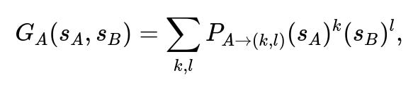
One major pitfall is that you need to carefully estimate the fraction of high influencers versus low influencers. Overestimating the proportion of high influencers can lead you to believe extinction is less likely. Another complexity is that type transitions can occur (a B user might become an A user if they gain influencer status), complicating the model further.
If there is a limit on maximum user capacity, does that guarantee eventual extinction or does it change the analysis?
Imposing a strict capacity (like a maximum N users, maybe due to infrastructure constraints) can transform the chain into a finite-state Markov chain with states {0,1,…,N}. In such a finite Markov chain, zero is often still absorbing if we define it that way, but the top capacity N might also be absorbing if the model forbids further growth beyond that point (or you might define transitions that keep the system near N).
Key difference: If the chain is truly irreducible except for zero being absorbing, you still can have a well-defined extinction probability. However, if there are multiple absorbing states (0 and N), you can have a chance to be stuck at capacity forever or eventually drop to zero. The exact probabilities of absorption in 0 or N can be computed by analyzing the chain’s transition matrix.
Pitfall: Some might conflate “reaching capacity” with indefinite success. If the chain can slip from N down to smaller states and eventually to zero, capacity is not truly absorbing unless you define it to be. Real systems might have partial fluctuations around that capacity. If you treat N as absorbing, you might get artificially low extinction probability. If you treat it as non-absorbing, you might get a more nuanced picture but a bigger modeling challenge.
In practical terms, how would you collect data to estimate the distribution for the single-user transitions?
You’d need detailed user-level event logs. For instance, for each user in your app, observe how many new users they attract (direct invites, viral shares, etc.) minus how many times they churn. Then you aggregate that data over many users/days to estimate P(X=k) for k=0,1,2,… Challenges include:
Not all invites are successful. You must separate “invitations sent” from “actual signups.”
Some new signups might come from external marketing rather than an existing user.
Some users churn slowly or remain inactive but not unsubscribed, blurring the definition of “spawned new users.”
Pitfalls:
• Sampling bias: If you track only active users, you might fail to see how effectively lapsed users bring in new signups after reactivation. • Time-lag: The new user might sign up days after receiving an invite, so attributing a user to a specific “parent user” might be tricky. • Underestimation of growth: Some new signups might not register that they were referred by an existing user (lack of referral codes).
How does the branching process approach compare to agent-based simulations in capturing user growth?
Branching processes assume each user spawns new users independently according to the same (or multi-type) distribution. Agent-based models can incorporate more nuanced behaviors, such as friend networks, social influence, and user-level preferences. An agent-based simulation might let each user see how many of their friends are on the platform, possibly leading to more correlated behaviors.
While branching processes are elegant and have closed-form or semi-closed-form solutions for extinction probabilities, agent-based models can show emergent phenomena (e.g., clusters of users forming strong communities, while others churn en masse). An agent-based approach might lead to a different extinction probability if local network effects are strong.
Pitfalls:
• Agent-based models can be computationally expensive and might require many runs to get stable estimates of extinction. • Overparameterization: You might introduce too many uncertain parameters (friend distribution, churn dynamics), making the model complex and less transparent. • Despite complexities, agent-based simulations often don’t provide simple closed-form solutions, so it’s harder to give exact probabilities of extinction without heavy Monte Carlo studies.
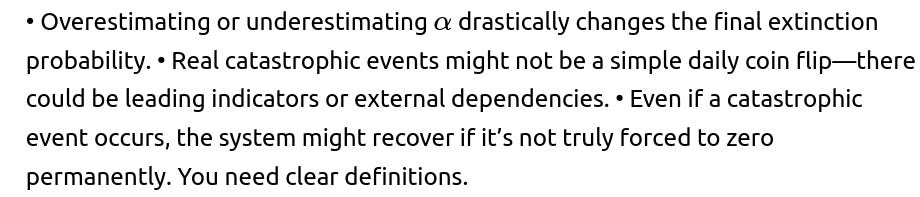
Could a single extreme event (like a security breach) overshadow the branching process analysis?
Yes. If there’s a small but non-negligible chance of a catastrophic event that instantly drives the user base to near zero (e.g., data leak, losing regulatory approval), that can dominate the extinction probability. A pure branching process or Markov chain typically deals with day-to-day transitions but might not incorporate rare catastrophic “shock events.” One way to include these:

Then the generating function approach has to be modified to factor in the random catastrophic event. The extinction probability can become significantly higher, especially over many days, because eventually that catastrophic event might happen.
Pitfalls:


How might business or product pivots alter the model assumptions?
If you pivot the app (e.g., from a social platform to a niche messaging tool), the fundamental user acquisition and retention dynamics can change. This is not captured by a stationary or even time-varying process with a single distribution. Instead, at some random time, the app might adopt new features that dramatically change user behavior. You effectively have piecewise definitions of the branching distribution:
Before pivot: P(X=k) is known.
After pivot: P(X=k) changes significantly.
One approach is to treat the pivot event as dividing your timeline. You compute the probability of extinction or survival up to the pivot, then condition on whether you survived at the pivot, and post-pivot you apply a new distribution. A major pitfall is that if the pivot is triggered by poor performance, you have endogeneity (the pivot might happen only if user counts are plummeting). Standard branching processes usually assume changes in distribution are exogenous or happen at fixed times, complicating the analysis if the pivot time depends on the user count.
How would you handle a scenario where the probability of moving from 1 user to 2 users also depends on how many times the app has already grown?
In real user growth, repeated expansions might get harder or easier. For instance, the first wave of invites could be simple (friends, family), but subsequent expansions might be more challenging as you run out of easy leads. This is a non-Markovian scenario because the transition probability from 1 user to 2 users depends not just on the current state (1 user) but also on the history (how many expansions have happened before).
You lose the memoryless property. You can model it as a more general state machine where your state includes both “current number of users” and “how many expansions have already occurred.” Then you have a Markov chain in a higher-dimensional state space, or you keep track of a “burnout factor” for each user. The branching process approach with a fixed distribution no longer suffices. You might have to code a custom simulation or derive a more elaborate chain-of-thought with an expanded Markov model.
Pitfalls:
• The dimensionality of states can blow up. • Trying to enforce a one-size-fits-all distribution might be misleading if real historical burn-in effects are strong.
In practical data science terms, how would you communicate this extinction probability result to stakeholders?
You’d likely present it as an estimate of “risk of complete user loss.” You’d emphasize that:
The result comes from an idealized model that assumes stationary growth probabilities.
The real risk might be higher or lower depending on marketing, competitor moves, and unpredictable shock events.
It still provides a valuable conceptual benchmark: if your estimated mean user growth per user is >1, you have a fighting chance of indefinite survival; if <1, your user base is doomed to vanish eventually.
Pitfalls in communication:
• Overstating the precision of your result. Stakeholders might interpret 1/6 as “exactly 16.6667%” chance of failure, but the real environment could deviate. • Neglecting to explain assumptions about stationarity and independence. If those assumptions break, the number is not reliable.
Could the extinction probability drop to zero if we tweak daily user-retention strategies slightly?
In theory, yes. If you adjust your product or marketing such that each user has a higher probability of bringing in more than one new user on average, you already have a supercritical branching process—but there can still be some nonzero chance of extinction. To drive that probability to zero, you’d need either:
• An infinitely large mean (unrealistic in practice). • A structure guaranteeing that from some state onward, you cannot decline to zero (e.g., guaranteed external marketing or mandated usage).
In real business, you might aim to raise the effective reproduction number enough to make extinction highly unlikely. But there will almost always remain a small chance that random fluctuations or external shocks drive the system to zero. So it’s rare to get the extinction probability truly to zero.
Pitfalls:
• Overconfidence: Even a strong supercritical process can still die out with small probability. • Short-term vs. long-term improvements: You might reduce short-term extinction risk but fail to account for variability in user behavior over time.
If the app starts with a different initial number of users, how do we compute the probability of eventual extinction?
For a Galton–Watson branching process, if you start with n users, the extinction probability is the probability that n independent branching lines each go extinct. If q is the extinction probability starting with 1 user, then for n independent users you get:


In more complex or correlated user-growth scenarios, that multiplication might not hold exactly because those lines may not remain independent (for instance, if multiple users overlap in the invites they send out). But in the simplest Galton–Watson scenario, that’s correct.
Pitfalls:


