
ML Interview Q Series: Prior vs. Posterior: Understanding Bayesian Belief Updating with Data

📚 Browse the full ML Interview series here.
Bayesian Prior vs Posterior: Explain the difference between a prior distribution and a posterior distribution in Bayesian inference. For instance, if you have a prior belief about the probability of an event and then observe new data, how do you update your belief to obtain the posterior?
Understanding Bayesian inference deeply revolves around how we represent our beliefs about unknown quantities (parameters or events) and how we update those beliefs when new evidence or data arrives. The framework uses “prior” and “posterior” distributions to capture these beliefs before and after observing data.
Bayesian inference is anchored in the idea that we have some initial assumption or “prior” about a parameter or event’s distribution. Then, after seeing observed data, we revise or update that assumption. This updated belief is known as the “posterior” distribution. Below is an in-depth explanation of each concept, the relationship between them, and potential follow-up discussions that might arise in a rigorous interview setting at a top technology company.
Heading for in-depth explanation (no numbering)
Prior Distribution
A prior distribution is a probability distribution that reflects our beliefs about a random variable (often a model parameter or an event’s probability) before we consider any new data. The term “prior” can sometimes be informed by domain knowledge, previous experiments, or purely subjective assumptions if we do not have much evidence. In more formal Bayesian terms:
The prior encapsulates what we think is plausible for the parameter’s values. If we are not very sure, we might pick a broad or non-informative prior that spans a wide range of values. If we already have strong reason to believe the parameter is near a certain region, we might choose a more concentrated prior.
In practice, the choice of prior can heavily influence the resulting posterior when data is limited. As the dataset grows large, the influence of the prior typically diminishes, and the observed data takes center stage.
Posterior Distribution
The posterior distribution is the probability distribution representing our updated belief about the parameter after seeing new data. Bayesian inference revolves around the concept of using observed evidence to adjust these beliefs. Intuitively:
We take the prior distribution and modify it by the likelihood of the observed data to obtain the posterior distribution.
This posterior not only tells us the most likely values of the parameter but also provides a measure of uncertainty (through its shape and spread).
Bayes’ Theorem and the Update Rule
The rigorous mechanism that relates prior and posterior is Bayes’ theorem. It essentially states that the posterior is proportional to the prior multiplied by the likelihood of the data under that prior assumption, all normalized by the evidence (or marginal likelihood).
Below is a typical expression of Bayes’ theorem. We center it and put it in H1 style with double dollar signs around it, as per instructions:

Where:
( \theta ) is the unknown parameter (or set of parameters).
( D ) is the observed data.
( P(\theta \mid D) ) is the posterior distribution over ( \theta ) after seeing data ( D ).
( P(D \mid \theta) ) is the likelihood function, describing how probable the observed data ( D ) is, given ( \theta ).
( P(\theta) ) is the prior distribution over ( \theta ).
( P(D) ) is the marginal likelihood or evidence, which ensures that the posterior distribution integrates (or sums) to 1.
Explanatory Notes:
“Posterior is proportional to Prior × Likelihood.” We often write ( P(\theta \mid D) \propto P(D \mid \theta), P(\theta) ) because ( P(D) ) is just a normalization term (it does not depend on ( \theta )).
The more new data we collect, the more the likelihood term ( P(D \mid \theta) ) typically reshapes and “updates” our belief about ( \theta ).
Example to Illustrate Prior and Posterior
Imagine you want to estimate the probability ( p ) of a coin landing heads. Before flipping it, you have some belief (prior) about ( p ). Perhaps you assume it’s a fair coin, so your prior is centered around ( p = 0.5 ), but you allow for some uncertainty, so you might choose a Beta distribution ( \mathrm{Beta}(2,2) ) that peaks near 0.5 yet spans (0,1).
Once you flip the coin several times, you observe, say, 8 heads and 2 tails. You use the likelihood (the binomial likelihood in this case) to update your prior. In a Beta-Binomial conjugate scenario:
Prior ( \mathrm{Beta}(\alpha, \beta) )
Posterior ( \mathrm{Beta}(\alpha + \text{number of heads}, \beta + \text{number of tails}) )
Hence if your prior was ( \mathrm{Beta}(2,2) ) and you see 8 heads and 2 tails, your posterior becomes ( \mathrm{Beta}(2 + 8,, 2 + 2) = \mathrm{Beta}(10,4). )
The updated posterior distribution shifts toward higher values of ( p ) because you observed more heads than tails.
Discussion of Posterior in Real-World Settings
In real-world scenarios where the model and parameter space are complex (e.g., deep neural networks with many parameters), deriving closed-form posteriors can be difficult. We often resort to approximate methods such as Markov Chain Monte Carlo (MCMC), Variational Inference, or Laplace Approximation to represent or sample from the posterior distribution.
Even if we cannot specify a perfect prior, we try to use some partial knowledge or we choose a non-informative / weakly informative prior. The primary goal is to ensure the model predictions reflect both the data and any prior domain knowledge in a balanced way.
Potential Tricky Points in an Interview Setting
Some might ask how sensitive a posterior can be to different priors. If the data is plentiful and of good quality, the posterior typically becomes more data-driven. If data is sparse, the choice of prior becomes critically important.
Another subtle point is “likelihood” vs. “posterior predictive.” In Bayesian inference, we might not only be interested in the distribution of ( \theta ) after seeing data but also in the predictive distribution of new data. The posterior distribution serves as the foundation for generating that posterior predictive distribution.
For real-world Bayesian deep learning, we often face high-dimensional parameter spaces. Techniques such as MC Dropout or Bayesian approximations attempt to glean uncertainty estimates that approximate the posterior’s spread.
Possible Implementation Sketch in Python
Below is a minimal example of a Bayesian update for a simple Bernoulli process, using a Beta prior.
import numpy as np
from scipy.stats import beta

# Suppose our prior for p is Beta(a_prior, b_prior).
a_prior = 2
b_prior = 2

# Observed data: let's say we have a record of heads and tails
# For demonstration, let's simulate some coin flips
np.random.seed(42)
coin_flips = np.random.binomial(1, 0.7, 10)  # 10 flips, p=0.7 for heads

heads_count = np.sum(coin_flips)
tails_count = len(coin_flips) - heads_count

# Posterior parameters for Beta distribution
a_post = a_prior + heads_count
b_post = b_prior + tails_count

print(f"Posterior parameters: a_post={a_post}, b_post={b_post}")

# We can do further analysis, e.g., posterior mean:
posterior_mean = a_post / (a_post + b_post)
print(f"Posterior mean for p = {posterior_mean}")

# We can also sample from the posterior:
samples = beta.rvs(a_post, b_post, size=10000)
print(f"Approx. 95% credible interval = [{np.percentile(samples,2.5)}, {np.percentile(samples,97.5)}]")
This snippet demonstrates how you start with a Beta(2,2) prior, update after observing coin flips, and then investigate the posterior distribution (its mean or credible interval).
Addressing Follow-Up Interview Questions
In an interview setting at a large tech company, simply reciting the difference between prior and posterior might not be enough. The interviewer often probes further to see if the candidate can handle tricky or deeply conceptual questions. Below are several potential follow-ups, each in H2 format, followed by thorough answers.
Could you discuss how the choice of prior affects the posterior when the amount of data is small vs. large?
When the dataset is small, the prior distribution can dominate because there is not enough empirical evidence to shift our belief drastically. This can be beneficial if we have well-founded domain knowledge encoded in the prior, or it can skew our results if our prior is not well-chosen.
As the dataset grows and more observations come in, the likelihood term typically overrides the influence of the prior. Even if the prior was somewhat off, a large volume of data will “pull” the posterior in the correct direction. This interplay highlights how Bayesian methods let us incorporate domain knowledge for situations where data is limited, and yet rely on data to guide inference when data is plentiful.
Potential Pitfalls:
Overly strong priors can “wash out” the data if the model tries to give excessive weight to the prior.
Too vague or flat priors can lead to computational issues or wide posterior distributions that do not reflect practical uncertainty bounds.
How does Bayesian updating work in high-dimensional models, such as neural networks?
In high-dimensional spaces (like modern deep neural networks), direct computation of the posterior becomes analytically intractable because we cannot express or integrate the high-dimensional likelihood easily. Instead, we rely on approximate Bayesian methods. Examples include:
Markov Chain Monte Carlo (MCMC): This samples from the posterior to approximate it with a set of draws. While theoretically exact given enough samples, it can be computationally expensive for very large models.
Variational Inference (VI): This technique posits a family of distributions (e.g., a fully factorized Gaussian) and tries to find the member of that family that best approximates the true posterior, typically by minimizing some divergence measure (like KL divergence).
Monte Carlo Dropout or Deep Ensembles: Heuristics used in Bayesian deep learning for approximate uncertainty estimation. The idea is that multiple runs or dropout-based sampling can approximate posterior uncertainty in predictions.
Why might practitioners prefer Bayesian approaches to frequentist methods?
Full distribution over parameters: Bayesian inference gives us a posterior distribution, not just a single estimate or confidence interval. This distribution can be directly used for predictive modeling and uncertainty quantification.
Domain knowledge encoding: Priors allow the inclusion of expert knowledge, which is extremely helpful when data is scarce or expensive.
Posterior predictive distributions: Bayesian methods yield a coherent framework to reason about future observations by integrating over all plausible parameters weighted by their posterior probabilities.
Potential concerns:
Computational overhead can be large.
Choosing priors can be subjective or non-trivial if domain knowledge is limited.
Is the posterior always guaranteed to be unimodal or well-behaved?
No, the posterior can be multimodal, skewed, or even improper (diverges under certain conditions). In complex models, sometimes local maxima in the likelihood can create multiple “regions” in parameter space that are similarly plausible. This complicates inference because naive methods might get stuck in one mode and fail to explore others. Techniques like advanced MCMC (e.g., Hamiltonian Monte Carlo with multiple chains) or specialized optimization methods in Variational Inference help address these complexities.
Could you discuss how Bayes’ theorem handles the normalizing constant ( P(D) ) in practice?
When we say:

the term ( P(D) ) (the marginal likelihood) is often a challenging integral:

For high-dimensional or complicated parameter spaces, this integral is not tractable. Methods like MCMC bypass the explicit calculation by sampling from the posterior in proportion to ( P(D \mid \theta),P(\theta). )
Variational inference also attempts to sidestep direct calculation of ( P(D) ) by optimizing a lower bound on the log evidence.
In simpler conjugate setups, we can often compute ( P(D) ) in closed form (e.g., Beta-Binomial, Normal-Gamma, etc.).
In what scenarios might you want to avoid or minimize subjective priors?
Although priors are fundamental to Bayesian methods, in some contexts you may not have reliable domain knowledge or you want to reflect a state of relative ignorance. You might then use:
Weakly informative priors that do not overly constrain the posterior.
Reference or Jeffreys priors, designed to yield posterior distributions with certain desired properties under transformation invariances.
However, even “uninformative” priors can be subtly informative. For instance, a uniform prior on one scale might not be uniform on a transformed scale. Hence, from a purely philosophical standpoint, every prior encodes some information, but you can attempt to reduce its influence.
How do Bayesian methods approach hypothesis testing compared to frequentist approaches?
In Bayesian hypothesis testing, you often compare model evidence or compute Bayes Factors: the ratio of marginal likelihoods for two competing hypotheses (models). For instance, if you have hypothesis ( H_0 ) vs. ( H_1 ), you compute:
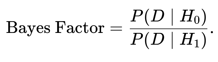
A large Bayes Factor > 1 in favor of ( H_0 ) means the data is more likely under ( H_0 ).
A small Bayes Factor < 1 indicates the data favors ( H_1 ).
This contrasts with p-values in frequentist approaches. Bayesian methods allow a more direct interpretation: you see how the posterior odds change from your prior odds in light of the data, clarifying which hypothesis the data supports.
How do you interpret a posterior predictive distribution?
Once you have a posterior distribution over parameters ( P(\theta \mid D) ), you can form a posterior predictive distribution for new data ( x_{\text{new}} ) by integrating over all possible ( \theta ). Symbolically:

This integral implies that you consider every possible parameter value, weighting it by how plausible it is after observing the data. The result is a predictive distribution that reflects both your updated best guess about the model parameter and the residual uncertainty in your parameter estimates. This is often considered one of the major advantages of Bayesian methods since it naturally includes uncertainty about parameters in the predictive step.
What might happen if the likelihood or prior is misspecified?
Bayesian methods rely on the assumption that the likelihood accurately represents the data-generating process and that the prior fairly encodes your beliefs or knowledge. If either is significantly off:
Misspecified Likelihood: If the model does not capture the true data dynamics, your posterior can systematically skew toward certain parameter values. This might lead to poor predictions, even if you collect more data.
Poor Prior: If your prior is extremely restrictive or misaligned with reality, it can distort your posterior in the regime of limited data. With more data, the effect of a poor prior typically diminishes, but this depends on how extreme the prior is.
How does one practically choose a prior?
The process can vary based on the problem setting:
Empirical Bayesian approaches: Estimate hyperparameters of the prior from the data itself (though this can be somewhat at odds with strict Bayesian principles).
Subject-Matter Expertise: In fields like medicine, astrophysics, or engineering, there might be well-established conventional priors based on decades of experimental results.
Non-informative or Weakly Informative: If you lack prior information, you might opt for distributions that are broad and let the data speak. Examples include wide normal priors for regression coefficients or half-Cauchy distributions for scale parameters.
If the prior is uniform, are we guaranteed to get a frequentist result?
In some basic cases (like a Beta prior for a Bernoulli process), a uniform prior on the parameter is the same as Beta(1,1). With enough data, the posterior might look close to the maximum likelihood estimate if we’re only examining the mean of the posterior. However, Bayesian approaches always maintain a distribution, so you will still have a posterior distribution that can differ from the frequentist confidence intervals or other constructs.
Could you highlight how real-life iterative Bayesian updates might work?
In certain applications—like online learning or real-time systems—you receive data in a streaming fashion. Bayesian methods allow you to recast the posterior after the first data batch as the new prior, then incorporate the next batch of data to obtain an updated posterior, and so on. This iterative update:
Start with prior ( P(\theta) ).
Observe data ( D_1 ), compute posterior ( P(\theta \mid D_1) ).
Use ( P(\theta \mid D_1) ) as the new prior for the next batch.
Observe data ( D_2 ), get ( P(\theta \mid D_1, D_2) ), and repeat.
This pipeline is elegant for evolving or non-stationary systems where data arrives incrementally.
Below are additional follow-up questions
How do we handle partial or mismatched prior knowledge in real-world scenarios?
In some practical use cases, you might only have strong domain knowledge about certain aspects of a problem, while other parts remain uncertain. For instance, you may know that a parameter should always remain positive and likely be below a certain threshold, but you lack clarity about its exact distribution. In such cases, you can impose an informative prior on that part of the parameter space you are more confident about and use a broader or less informative prior elsewhere.
A potential pitfall is applying an overly restrictive prior to parts of the model where your domain knowledge is not fully accurate. If the real-world conditions violate your assumptions, you risk biasing the posterior or ending up with a posterior that is “locked in” to unrealistic parameter values when data is sparse. As you collect more data, any mismatch might be partially mitigated, but severe inconsistencies may still persist.
Another edge case arises when the prior is so radically misaligned with the data that the posterior ends up skewed or heavily bimodal. In some instances, advanced sampling methods might fail to converge (the chain can jump erratically or remain stuck in a small region). Addressing this requires either reevaluating the prior’s assumptions or collecting additional data to clarify the parameter space.
What if the data is extremely high dimensional or complex?
When data is high dimensional or you are dealing with complicated models (for example, involving latent variables or high-dimensional feature spaces), the likelihood can be difficult to evaluate. Bayesian updating then faces steep computational costs. Techniques for approximate inference, including Variational Inference or advanced Markov Chain Monte Carlo algorithms like Hamiltonian Monte Carlo, can help manage the complexity.
Pitfalls arise when the dimensionality of the parameter space outpaces the sampling or optimization capabilities. MCMC chains may mix poorly across vast parameter regimes. Variational approximations might adopt simplifications (like mean-field assumptions) that fail to capture critical dependencies, causing the posterior to be systematically underdispersed or missing certain important correlations.
Edge cases happen if the data has many redundant or irrelevant features. Bayesian methods might allocate significant posterior probability mass to certain parameter configurations that explain spurious correlations. Proper regularization via careful priors, dimension reduction, or domain-driven constraints can help mitigate these issues.
What if we have to handle a continually changing environment and keep updating our posterior?
In dynamic or non-stationary environments, the data distribution can shift over time. Standard Bayesian inference typically assumes the data is drawn from the same underlying distribution. To keep the model updated in a shifting environment, you can employ:
Bayesian online learning: Each posterior becomes the prior for the next time step. However, if the data distribution fundamentally changes, the old posterior might not properly represent the new reality.
Sliding window or forgetting mechanisms: Give higher weight to more recent data, effectively “discounting” older observations so that the posterior remains responsive to changes.
Time-varying or hierarchical models: Explicitly model temporal evolution of parameters via state-space methods or hierarchical frameworks that update parameters in a manner consistent with potential drift over time.
A possible pitfall is overreacting to short-term fluctuations. If the environment changes slowly, an aggressive forgetting factor might discard valuable historical data. Conversely, too conservative an approach might make the posterior adapt too slowly. Tuning this trade-off often requires domain insights and empirical testing on real data streams.
How do we deal with situations where the posterior distribution might not converge?
In well-behaved Bayesian problems with consistent data and a coherent model, the posterior generally concentrates around the true parameter values as data grows. However, there are scenarios where the posterior may fail to converge or converge extremely slowly:
Model misspecification: If the assumed likelihood significantly deviates from the actual data-generating process, the posterior might never concentrate on a correct set of parameters.
Incompatible priors: Certain priors might place negligible probability around the true parameter values, preventing the posterior from covering them effectively, especially with limited data.
Multi-modal or pathological likelihood surfaces: MCMC-based sampling could have trouble exploring all modes, leading to partial exploration and poor convergence diagnostics.
Practically, it is crucial to monitor convergence indicators (e.g., Gelman–Rubin statistic for MCMC, or evidence-based measures). Re-examining the model, collecting more data, or adjusting the sampling algorithms are all typical strategies for diagnosing or fixing convergence issues.
Could you elaborate on the difference between the full posterior distribution and point estimates like the MAP?
While the full posterior distribution captures every possible value of the parameter along with its associated probability (reflecting uncertainty), a maximum a posteriori (MAP) estimate picks out a single parameter value that maximizes the posterior. This is often found by taking the negative log of the posterior and using gradient-based optimization.
A key difference is that MAP discards the rich spread of uncertainty in the posterior, focusing solely on the most probable point. This can be acceptable if you only need a single estimate and the posterior is fairly peaked. But in cases where you need uncertainty quantification—such as risk assessment in mission-critical domains—using the entire posterior is more informative.
An edge case is when the posterior is multi-modal. MAP could land in a local maximum and miss more globally relevant modes. A full posterior perspective reveals all modes and their relative probabilities, helping you better understand the potential solutions.
When might a Bayesian credible interval differ substantially from a frequentist confidence interval?
A credible interval directly represents the posterior probability that the parameter lies in a certain range. A frequentist confidence interval is a procedure-based interval that, if repeated many times, will contain the true parameter a certain percentage of the time. Although credible intervals often numerically resemble confidence intervals for large sample sizes, they can differ markedly in small-sample or highly informative-prior situations.
One subtle scenario is if you have a very strong prior that is not centered around the frequentist estimate. The Bayesian credible interval may be shifted or narrower due to that prior information. Meanwhile, a frequentist confidence interval typically does not incorporate such knowledge and might be wider or differently shaped based solely on the likelihood from the data.
Pitfalls arise in interpreting confidence intervals as if they were Bayesian statements about the probability of containing the parameter. Such an interpretation is incorrect in frequentist statistics but is precisely how one can interpret a Bayesian credible interval.
How do we handle large data sets in Bayesian inference without incurring enormous computational overhead?
For massive data sets, the cost of evaluating the likelihood for every observation in each iteration of MCMC can become prohibitive. Several strategies address this challenge:
Stochastic Variational Inference: Uses mini-batches of data to update an approximate posterior in an iterative fashion.
Stochastic Gradient MCMC (e.g., Stochastic Gradient Langevin Dynamics): Incorporates gradient information from random subsets of data to approximate posterior sampling.
Divide-and-Conquer Techniques: Partition the data into subsets, run parallel Bayesian updates, and then combine the posterior approximations using methods designed for distributed settings.
A potential pitfall is that approximate or distributed methods may lose accuracy or induce bias, especially if the data partitions are not representative of the overall distribution. Careful sampling or weighting may be required to mitigate these risks.
How do hierarchical or multi-level priors influence the posterior?
Hierarchical Bayesian modeling introduces another layer of parameters, often called hyperparameters, which govern the priors for lower-level parameters. For example, in a multi-level model of multiple experimental units, each unit might have a local parameter, but these local parameters share a hyperprior that enforces partial pooling across units.
In these models:
Each level’s posterior depends on the priors or hyperpriors above it.
Data from different units can inform each other indirectly by updating the hyperparameters, which then shift or constrain the local-level posteriors.
A common pitfall is that hierarchical models can be quite sensitive to the choice of hyperprior if data is scarce. Conversely, if data is plentiful across many units, a hierarchical framework can greatly improve inference by leveraging shared information. Convergence can be trickier; multi-level structures introduce correlations between layers, and naive MCMC methods might mix poorly if the dimensionality grows large.
How do robust Bayesian methods deal with outliers or heavy-tailed distributions?
A standard Gaussian likelihood may be vulnerable to outliers, as a few extreme data points can disproportionately alter the posterior, particularly when the prior is not strongly controlling the tails. Robust Bayesian methods might use:
Heavy-tailed likelihoods (e.g., Student’s t distribution) to reduce the influence of large residuals.
Mixture models that explicitly allow a small fraction of outlier data to be explained by a separate distribution.
Priors structured in a way that impose cautious updates in the presence of suspicious data.
A subtle edge case occurs if your data includes systematic anomalies rather than random outliers. Merely adopting a robust likelihood will not automatically fix the mismatch, especially if the anomalies represent a meaningful component of the data generating process. In such scenarios, a carefully designed model that includes an outlier or contamination component can prevent the main posterior from being distorted.
How do we incorporate non-traditional forms of evidence (like expert statements) into a prior?
Sometimes you have experts providing statements about possible parameter ranges or relationships. For example, a doctor might say, “In nearly all patients, the effect of this drug should not exceed a certain dosage effect.” Translating qualitative or soft constraints into a prior can involve:
Using a bounding prior that heavily penalizes parameter values beyond stated thresholds.
Transforming statements about likelihood of success or risk levels into a Beta or normal distribution parameterization.
An edge case arises when multiple experts disagree or provide conflicting statements. You could combine their opinions into a mixture prior, weighting each expert’s input. Alternatively, you may run separate analyses under each expert’s prior to see how the posterior changes (a sensitivity analysis). Care must be taken that these subjective priors do not overshadow strong empirical trends if you do eventually observe data that contradicts the experts’ positions.
Why do conjugate priors matter, and do they still matter in modern large-scale Bayesian inference?
Conjugate priors are chosen such that the posterior remains in the same parametric family as the prior. A classic example is the Beta prior for a Bernoulli likelihood, yielding a Beta posterior. This can be mathematically elegant and computationally efficient because updating the posterior requires only analytical formulae.
In modern large-scale or high-dimensional Bayesian tasks, conjugacy is often not feasible due to more complicated likelihoods. Nonetheless, conjugate or semi-conjugate priors remain useful in simpler submodules of a larger model, or for quick updates in streaming situations where real-time computation is essential. They also serve as good pedagogical examples or baseline approaches before introducing more advanced approximate methods. In some edge cases, specifically engineered model components can preserve partial conjugacy and thereby simplify the inference steps for certain parameters.
What are practical concerns for validating a Bayesian model’s posterior?
A Bayesian model can be validated by checking whether the posterior predictions align with observed data and domain knowledge. Techniques like posterior predictive checks allow you to:
Sample new data points from the posterior predictive distribution.
Compare those generated samples to actual observations to see if they look qualitatively similar or if there are systematic discrepancies.
You can also use scoring rules (like the log predictive density on held-out data) to quantify predictive accuracy. However, pitfalls appear when the model is substantially mis-specified or if the prior strongly biases certain outcomes. Merely “fitting the data well” does not guarantee that the posterior is capturing the right structure if you used a flexible but misspecified likelihood. Sensitivity analyses—varying priors or removing subsets of data—can help highlight how robust your posterior is to specific assumptions.