


ML Interview Q Series: Probability Calculations for Normal Variables via Standardization

Browse all the Probability Interview Questions here.
Suppose X is N(-1, 4). Find (a) P(X < 0), (b) P(X > 1), (c) P(-2 < X < 3), (d) P(|X+1| < 1).
Short Compact solution
From the fact that X can be written as X = 2Z + 1, where Z is a standard normal random variable:
P(X < 0) = P(2Z + 1 < 0) = P(Z < -1/2) = Φ(-1/2) = 1 – Φ(1/2) ≈ 0.3085
P(X > 1) = P(2Z + 1 > 1) = P(Z > 0) = 1 – Φ(0) = 1 – 0.5 = 0.5
P(-2 < X < 3) = P(-2 < 2Z + 1 < 3) = P(-3/2 < Z < 1) = Φ(1) – Φ(-3/2) ≈ 0.7745
P(|X + 1| < 1) = P(-2 < X < 0) = P(-3/2 < Z < -1/2) = Φ(-1/2) – Φ(-3/2) ≈ 0.2417
Comprehensive Explanation
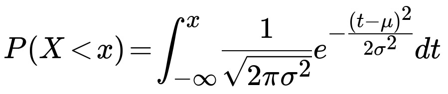
Understanding the distribution of X X is given to be normally distributed with mean -1 and variance 4. Equivalently, X ~ N(-1, 4). The standard approach to handle probabilities involving a normally distributed variable is to convert X to its standardized form involving the standard normal variable Z, which has mean 0 and variance 1.
where
μ is the mean of X (which is -1),
σ is the standard deviation of X (the square root of 4, which is 2),
Z is a standard normal variable (Z ~ N(0,1)).
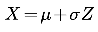
Hence, we can write X as X = -1 + 2Z.
By substituting X = -1 + 2Z, each probability can be turned into an event about the standard normal variable Z, for which tables or standard library functions (e.g., scipy.stats.norm.cdf in Python) are typically used.
1. Probability P(X < 0)
We need P(X < 0). Using X = -1 + 2Z, the event X < 0 is:
-1 + 2Z < 0 2Z < 1 Z < 1/2 multiplied by 1/2? Let's be careful:
Actually, rearranging -1 + 2Z < 0: 2Z < 1 (by adding 1 to both sides) Z < 1/2
But from the short solution we see it done as 2Z + 1 < 0 => 2Z < -1 => Z < -1/2. Let us verify carefully:
Given X = 2Z + 1, "X < 0" is the same as 2Z + 1 < 0, so
2Z < -1 Z < -1/2
Hence
P(X < 0) = P(Z < -1/2).
The quantity P(Z < -1/2) can be expressed using the standard normal cumulative distribution function Φ:
P(Z < -1/2) = Φ(-1/2).
Because the standard normal is symmetric, Φ(-1/2) = 1 – Φ(1/2). Numerically, Φ(1/2) is about 0.6915, so we get P(X < 0) ≈ 1 – 0.6915 = 0.3085.
2. Probability P(X > 1)
We want P(X > 1). With X = 2Z + 1:
2Z + 1 > 1 2Z > 0 Z > 0
Thus P(X > 1) = P(Z > 0). Because Z is standard normal, P(Z > 0) = 1 – Φ(0) = 1 – 0.5 = 0.5.
3. Probability P(-2 < X < 3)
We look at the double inequality:
-2 < X < 3 -2 < 2Z + 1 < 3
Subtract 1 from all parts:
-3 < 2Z < 2
Divide everything by 2:
-3/2 < Z < 1
Hence,
P(-2 < X < 3) = P(-3/2 < Z < 1) = Φ(1) – Φ(-3/2).
Using standard normal tables or software, Φ(1) ≈ 0.8413 and Φ(-3/2) = 1 – Φ(3/2). Numerical value of Φ(3/2) is about 0.9332, so Φ(-3/2) ≈ 0.0668. Therefore
P(-2 < X < 3) ≈ 0.8413 – 0.0668 = 0.7745.
4. Probability P(|X + 1| < 1)
This involves the absolute value condition |X + 1| < 1. That is equivalent to:
-1 < X + 1 < 1
Subtract 1 throughout:
-2 < X < 0
We already know X = 2Z + 1. Substitute:
-2 < 2Z + 1 < 0
Subtract 1 from all sides:
-3 < 2Z < -1
Divide by 2:
-3/2 < Z < -1/2
So
P(|X + 1| < 1) = P(-3/2 < Z < -1/2) = Φ(-1/2) – Φ(-3/2).
Using numerical values, Φ(-1/2) = 1 – Φ(1/2) ≈ 1 – 0.6915 = 0.3085, and Φ(-3/2) = 1 – Φ(3/2) ≈ 1 – 0.9332 = 0.0668. Hence
P(|X + 1| < 1) ≈ 0.3085 – 0.0668 = 0.2417.
These results match the short compact solution provided.
Potential Follow-up Question 1: How do we interpret the standardization procedure in practical terms?
When we say X ~ N(μ, σ²), we can express X as μ + σZ, where Z ~ N(0,1). The transformation Z = (X – μ)/σ is called the standardization of X. In practice, if one has a normal random variable X with known mean and standard deviation, any question about its probability over an interval reduces to looking up or computing areas under the standard normal distribution curve for certain bounds. This standardization step is crucial because tables and built-in functions commonly exist only for the standard normal distribution.
In real-world tasks, for example, if X represents a measurement such as height or weight (often approximated by a normal distribution), standardization allows direct comparison with standard normal thresholds. Probability statements about X can then be found using standard normal cumulative distribution tables or software libraries.
Potential Follow-up Question 2: Why does symmetry help us rewrite Φ(-a) in terms of Φ(a)?
The standard normal distribution is symmetric about 0. For a standard normal variable Z:
P(Z < -a) = P(Z > a)
because reflecting around 0 makes the negative side mirror to the positive side. Hence,
Φ(-a) = 1 – Φ(a).
This is simply a consequence of the shape of the bell curve, centered at 0, meaning that the amount of probability mass below -a is the same as the amount of probability mass above +a.
Potential Follow-up Question 3: How would we compute these probabilities in Python?
You can use the scipy.stats library, specifically the norm object which has CDF (.cdf) and PDF (.pdf) methods. As a quick illustration:
import numpy as np
from scipy.stats import norm

# Mean and standard deviation
mu = -1
sigma = 2

# 1. P(X < 0)
p1 = norm.cdf((0 - mu) / sigma)  # standardizing
print("P(X<0) =", p1)

# 2. P(X > 1)
p2 = 1 - norm.cdf((1 - mu) / sigma)
print("P(X>1) =", p2)

# 3. P(-2 < X < 3)
p3 = norm.cdf((3 - mu) / sigma) - norm.cdf((-2 - mu) / sigma)
print("P(-2<X<3) =", p3)

# 4. P(|X+1|<1) --> -2 < X < 0
p4 = norm.cdf((0 - mu) / sigma) - norm.cdf((-2 - mu) / sigma)
print("P(|X+1|<1) =", p4)
The values you get will closely match those from the solution steps above.
Potential Follow-up Question 4: What happens if X has correlations with other variables?
If X is part of a jointly normal vector (X, Y, ...), then X itself is still normally distributed if the joint distribution is multivariate normal. You can still talk about P(X < a) in the same manner. However, if you need joint probabilities such as P(X < a, Y < b), you must consider the correlation structure between X and Y. In that setting, standardization would require you to account for covariances and you may need to use the multivariate normal CDF or transformations that incorporate correlation (for example, using Cholesky decompositions). Standard normal tables are not sufficient for higher-dimensional integrals, and one often relies on numerical methods or specialized libraries to compute multivariate normal probabilities.
Potential Follow-up Question 5: Could we have computed these probabilities using the PDF of the normal distribution directly?
While one can in principle integrate the PDF of X from the relevant lower bound to upper bound, that integral is exactly what the CDF function does. In other words, you would write:
In practice, direct integration is usually bypassed, and tables or software for Φ (the standard normal CDF) are used. Hence the typical workflow is:
Convert X to the standard normal form Z.
Use the known standard normal CDF Φ(z).
This approach is more efficient and less error-prone than attempting to do the integral manually each time, especially when dealing with multiple bounds.