
ML Interview Q Series: Probability Density and Moments of Triangle Area (V = \tfrac{1}{2} \tan(\Theta)) for Uniform (\Theta).
Browse all the Probability Interview Questions here.
Short Compact solution
We define the area of the triangle by (V = \tfrac12 \tan(\Theta)). Because (\Theta) is uniformly distributed on ((0,\tfrac{\pi}{4})) with density (4/\pi), one can compute:
[
\huge E(V) ;=; \tfrac12 \int_{0}^{\pi/4} \tan(\theta) ,\tfrac{4}{\pi},d\theta ;=; \tfrac{1}{\pi},\ln(2), ] and [ \huge E(V^{2}) ;=; \tfrac14 \int_{0}^{\pi/4} \tan^{2}(\theta),\tfrac{4}{\pi},d\theta ;=; \tfrac1\pi,\Bigl(1 - \tfrac{\pi}{4}\Bigr). ] Hence, the standard deviation is [ \huge \sqrt{;E(V^2);-;\bigl(E(V)\bigr)^2},. ] By change of variables (V = \tfrac12 \tan(\theta)), we get (\theta = \arctan(2,V)). The derivative (d\theta/dV = 2/(1+4,V^2)) then gives the probability density of (V) as [ \huge f_{V}(v) ;=; \tfrac{8}{\pi ,\bigl(1 + 4,v^2\bigr)} \quad \text{for } 0 < v < \tfrac12. ]
Comprehensive Explanation
Geometry of the problem
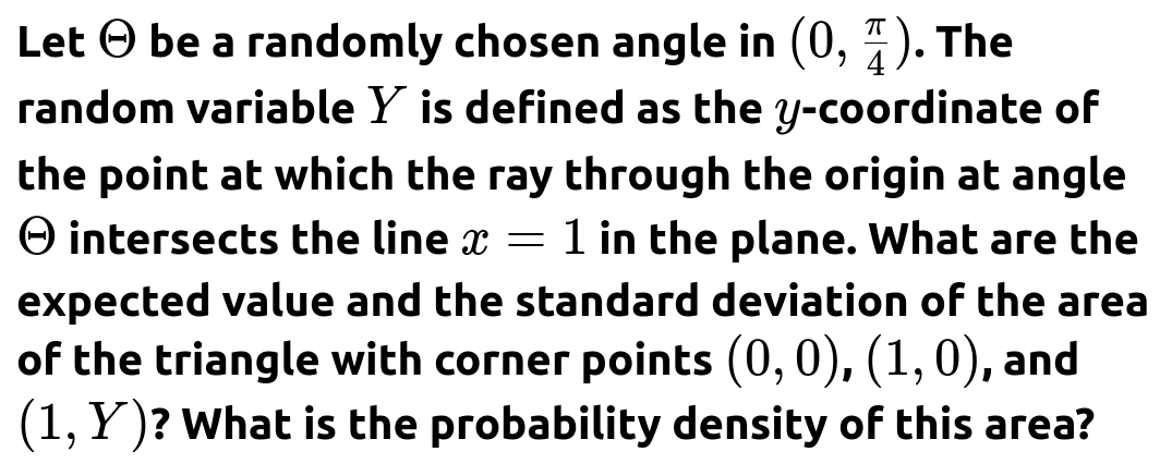
We have a random angle (\Theta) drawn uniformly from the interval ((0,\tfrac{\pi}{4})). In the ((x,y)) plane, we draw a ray from the origin ((0,0)) at angle (\Theta). This ray intersects the vertical line (x=1) at some point ((1,Y)). Because (\tan(\Theta) = Y/1), the (y)-coordinate of this intersection point is (Y = \tan(\Theta)).
Area of the triangle
We look at the triangle formed by the points ((0,0)), ((1,0)), and ((1,Y)). This triangle has base 1 (on the (x)-axis between ((0,0)) and ((1,0))) and height (Y). Hence its area (V) is given by
The random variable (V) therefore depends on (\Theta) via the tangent function.
Distribution of (\Theta)
Since (\Theta) is chosen uniformly from ((0,\tfrac{\pi}{4})), the probability density function for (\Theta) is
[
\huge f_{\Theta}(\theta)
\begin{cases} \tfrac{4}{\pi} & 0 < \theta < \tfrac{\pi}{4},\ 0 & \text{otherwise}. \end{cases} ]
The factor (4/\pi) ensures the total probability integrates to 1 over ((0,\tfrac{\pi}{4})).
Expected area (E(V))
To find the expected value (E(V)), we use the definition of expectation for a continuous random variable:
[
\huge E(V)
\int_{-\infty}^{\infty} v,f_{V}(v),dv
\int_{0}^{\pi/4} \bigl(\tfrac12\tan(\theta)\bigr), f_{\Theta}(\theta), d\theta, ] since (V=\tfrac12 \tan(\theta)) and (\Theta) only takes values in ((0,\tfrac{\pi}{4})). Substituting (f_{\Theta}(\theta)=\tfrac{4}{\pi}), we get
$$ E(V)
;=; \tfrac12 \int_{0}^{\pi/4} \tan(\theta),\tfrac{4}{\pi},d\theta ;=; \tfrac{2}{\pi}\int_{0}^{\pi/4} \tan(\theta),d\theta ;=; \tfrac{1}{\pi},\ln\bigl(\sec(\theta)\bigr)\Big|_{0}^{\pi/4}. $$
Evaluating (\ln(\sec(\theta))) from 0 to (\pi/4) gives (\ln(\sec(\pi/4)) - \ln(\sec(0)) = \ln(\sqrt{2}) - \ln(1) = \ln(\sqrt{2}) = \tfrac12\ln(2)). That yields
Second moment and variance of (V)
We next compute (E(V^2)). This is
[
\huge E(V^2)
\int_{0}^{\pi/4} \bigl(\tfrac12\tan(\theta)\bigr)^2,f_{\Theta}(\theta),d\theta
\tfrac14 \int_{0}^{\pi/4} \tan^2(\theta),\tfrac{4}{\pi},d\theta
\tfrac{1}{\pi}\int_{0}^{\pi/4} \tan^2(\theta),d\theta. ]
We use the identity (\tan^2(\theta)=\sec^2(\theta)-1) and integrate:
[ \huge \int_{0}^{\pi/4} \tan^2(\theta),d\theta
\int_{0}^{\pi/4} \bigl[\sec^2(\theta)-1\bigr],d\theta
\bigl[\tan(\theta)\bigr]_{0}^{\pi/4}
\bigl[\theta\bigr]_{0}^{\pi/4}
1 - \tfrac{\pi}{4}. ]
Hence
$$ E(V^2)
;=; \tfrac{1}{\pi},\Bigl(1 - \tfrac{\pi}{4}\Bigr). $$
The variance of (V) follows as
$$ \text{Var}(V)
;=; E(V^2);-;\bigl(E(V)\bigr)^2. $$
Thus
[ \huge \text{Var}(V)
\tfrac{1}{\pi}\Bigl(1-\tfrac{\pi}{4}\Bigr) -\Bigl(\tfrac{1}{\pi}\ln(2)\Bigr)^2. ]
Finally, the standard deviation is the square root of this variance.
Probability density of (V)
We find (f_{V}(v)) using the standard transformation approach. Given
[
\huge v
\tfrac12 \tan(\theta), ] we solve for (\theta):
[ \huge \theta
\arctan(2,v). ]
Because (v) ranges from 0 to (\tfrac12\tan(\tfrac{\pi}{4})=\tfrac12) when (\theta) goes from 0 to (\tfrac{\pi}{4}), the support of (V) is ((0,\tfrac12)). The derivative is
[ \huge \tfrac{d\theta}{dv}
\tfrac{2}{1+4,v^2}. ]
Therefore,
[
\huge f_{V}(v)
f_{\Theta}\bigl(\arctan(2,v)\bigr), \bigl|\tfrac{d}{dv}\arctan(2,v)\bigr|
\tfrac{4}{\pi}\times \tfrac{2}{1+4,v^2}, ] which simplifies to
$$ f_{V}(v) ;=; \tfrac{8}{\pi,\bigl(1 + 4,v^2\bigr)}
\quad \text{for } 0 < v < \tfrac12. $$
That completes the full characterization of the distribution of (V).
Possible Follow-Up Questions
Why does (\Theta) have density (4/\pi) on (\bigl(0,\tfrac{\pi}{4}\bigr)) instead of (\tfrac{1}{\pi/4})?
When a random variable is said to be chosen uniformly from (\bigl(0,\tfrac{\pi}{4}\bigr)), the length of that interval is (\pi/4). A uniform density on that interval is (1 / (\tfrac{\pi}{4})=4/\pi). This ensures that integrating the density from 0 to (\pi/4) gives 1.
What if the angle was chosen uniformly in (\bigl(0,\tfrac{\pi}{2}\bigr))?
Then the density would be (f_{\Theta}(\theta)=\tfrac{2}{\pi}) for (\theta\in\bigl(0,\tfrac{\pi}{2}\bigr)). The derived formulas for (V=\tfrac12 \tan(\Theta)) would change accordingly, and (V) would then range from 0 to (\infty). You would re-do the integrals and find a very different expectation and variance, and the probability density of (V) would also be supported on all positive real numbers.
How to interpret this area distribution in practice?
Geometrically, each angle (\Theta) leads to a specific triangle of base 1 and height (\tan(\Theta)). Because (\Theta) is limited to (\bigl(0,\tfrac{\pi}{4}\bigr)), the tangent remains below 1, so the maximal area is (\tfrac12). The area thus never exceeds 0.5, and the probability density (f_{V}(v)) explains how likely each area value is, with more likelihood near smaller areas but a decently high chance of areas near 0.5 as well—governed by the (\tfrac{1}{1+4,v^2}) shape.
Why does (V) range only between 0 and (\tfrac12)?
When (\theta=0), (\tan(\theta)=0), so the area (V) is 0. When (\theta=\tfrac{\pi}{4}), (\tan(\theta)=1), and thus (V=\tfrac12). So the random variable (V=\tfrac12 \tan(\Theta)) indeed takes values strictly between 0 and 0.5.
Can you show a quick Python snippet to sample from this distribution?
Below is an illustrative code example using inverse transform sampling. We first draw (\Theta\sim\text{Uniform}(0,\tfrac{\pi}{4})), then compute (V=\tfrac12 \tan(\Theta)):
import numpy as np

def sample_area(n_samples=10_000_000):
    # Sample Theta uniformly in (0, pi/4)
    theta_samples = np.random.uniform(0, np.pi/4, size=n_samples)
    # Compute V = 1/2 * tan(Theta)
    V_samples = 0.5 * np.tan(theta_samples)
    return V_samples

# Example usage
V_data = sample_area()
print("Approx mean:", np.mean(V_data))
print("Approx std:", np.std(V_data))
For a large number of samples, this should approximate the theoretical results (E(V)=\tfrac{1}{\pi}\ln(2)) and the standard deviation computed from the exact variance formula above.
Below are additional follow-up questions
What if we shift the angle domain slightly, for example (\Theta \in (\pi/8, \pi/4)), instead of ((0, \pi/4))? How would that affect the expected area and the distribution of (V)?
If we restrict (\Theta) to lie in a smaller interval, say (\bigl(\tfrac{\pi}{8}, \tfrac{\pi}{4}\bigr)), then the density of (\Theta) would no longer be (4/\pi). Instead, for a uniform distribution on (\bigl(\tfrac{\pi}{8}, \tfrac{\pi}{4}\bigr)), the density would be (1 / \bigl(\tfrac{\pi}{4}-\tfrac{\pi}{8}\bigr) = 1 / \bigl(\tfrac{\pi}{8}\bigr) = 8/\pi). As a result:
The range of (V) would also shift. If (\Theta\in \bigl(\tfrac{\pi}{8}, \tfrac{\pi}{4}\bigr)), then
The minimum of (V) would be (\tfrac12 \tan(\tfrac{\pi}{8})).
The maximum of (V) would remain (\tfrac12 \tan(\tfrac{\pi}{4})= \tfrac12).
The expected area (E(V)) would be an integral of (\tfrac12\tan(\theta)) over (\theta\in(\tfrac{\pi}{8}, \tfrac{\pi}{4})) with the updated density (8/\pi). Numerically, this typically yields a larger average (V) than if (\Theta) started from 0 because we exclude smaller angles.
The probability density (f_{V}(v)) would also be derived by the same transformation logic (v = \tfrac12\tan(\theta)) but with different integration limits. Essentially, the entire distribution would “shift” or re-scale to reflect the narrower range of angles.
A potential pitfall is forgetting to normalize the density properly when you change the domain. You must carefully integrate over the correct limits and use the correct uniform density. Also, you need to remember that the support of (V) is no longer ((0,\tfrac12)) but rather (\bigl(\tfrac12\tan(\tfrac{\pi}{8}), \tfrac12\bigr)).
If (\Theta) were allowed to take values outside ((0,\pi/4)), like negative angles or angles larger than (\pi/4), how would that affect the triangle area?
Let’s consider two scenarios:
Negative angles: If (\Theta < 0), then (\tan(\Theta)) could be negative. In a strict geometric sense, if you shoot a ray at a negative angle in the plane (i.e., below the x-axis), you’d still intersect (x=1) at some point, but its (y)-coordinate would be negative. This would mean the “triangle” we are trying to form either has zero or negative area if we keep using (\tfrac12 \tan(\Theta)). You’d have to redefine the concept of “area” to ensure it’s always nonnegative—typically by taking the absolute value of the height or restricting the domain to (\Theta\ge 0).
Angles beyond (\pi/4): For (\Theta>\pi/4), we’d have (\tan(\Theta) > 1). This would make the point of intersection at ((1,Y)) with (Y>1), so the area can exceed (\tfrac12). If the domain for (\Theta) was, say, ((0,\pi/2)), (V) could become arbitrarily large as (\Theta\to \tfrac{\pi}{2}). You’d need to redo the integrals carefully for (\Theta\in(0,\tfrac{\pi}{2})).
A subtle pitfall is failing to consider the sign of (\tan(\Theta)) if (\Theta) extends beyond ((-\tfrac{\pi}{2},\tfrac{\pi}{2})). In real-world geometric interpretations, you typically want a nonnegative area, so domain restrictions are crucial.
Could we have derived the distribution of (V) from a purely geometric viewpoint without using the transformation formula?
Yes, a purely geometric viewpoint might proceed as follows:
Recognize that (\Theta) is uniform in ((0,\tfrac{\pi}{4})). This means that if you draw all possible rays from the origin within that wedge, they are “equally likely” in angular measure.
Observe that (V=\tfrac12 \tan(\Theta)) can be seen as half the ratio (\frac{Y}{X}) where (X=1). As (\Theta) increases, the area grows from 0 up to \tfrac12.
You could directly calculate the fraction of angles leading to an area (\leq v). Namely, you want (\tfrac12\tan(\Theta)\leq v) or (\theta \le \arctan(2v)). Since (\Theta) is uniform, the CDF (F_V(v)) is the ratio of that angular measure to the total measure (\tfrac{\pi}{4}).
Differentiate the CDF to find the PDF.
A potential pitfall is mixing up the geometric measures (arc length or sector area) with angles. One might mistakenly assume a uniform distribution in terms of radial lines or lengths, whereas here we are uniform in angle measure. Always confirm which measure of uniformity applies.
What if we replaced the line (x=1) with the line (x=c) for some constant (c>0)? How does that change the area distribution?
In that case, the point of intersection becomes ((c,,Y)) with (Y = c\tan(\Theta)). Then the area of the triangle with vertices ((0,0)), ((c,0)), and ((c,Y)) would be
[
\huge V
\tfrac12 \times \text{(base)} \times \text{(height)}
\tfrac12 \times c \times \bigl(c \tan(\Theta)\bigr)
\tfrac{c^2}{2},\tan(\Theta). ]
The logic behind computing moments and distributions is identical, but each instance of (\tfrac12 \tan(\Theta)) is replaced by (\tfrac{c^2}{2}\tan(\Theta)). Key changes:
The maximum possible area (when (\Theta\to \pi/4)) becomes (\tfrac{c^2}{2}\cdot 1 = \tfrac{c^2}{2}).
The support of (V) is ((0,,\tfrac{c^2}{2})).
The transformation formula for (v = \tfrac{c^2}{2}\tan(\theta)) changes to (\theta=\arctan\bigl(\tfrac{2v}{c^2}\bigr)).
The Jacobian becomes (\tfrac{d\theta}{dv}=\tfrac{2}{c^2,(1+(\tfrac{2v}{c^2})^2)}), leading to a different PDF but with a similar shape.
A subtlety here is if (c\le0). That would disrupt the geometry of the “triangle” in question or invert the axis orientation. Typically, we assume (c>0).
How would we compute higher-order moments (e.g., (E(V^3)) or (E(V^4))) if needed for skewness or kurtosis?
To find (E(V^n)), you would proceed with the integral:
[
\huge E(V^n)
\int_{0}^{\pi/4} \Bigl(\tfrac12\tan(\theta)\Bigr)^n f_{\Theta}(\theta),d\theta. ]
For a uniform (\Theta \in (0,\tfrac{\pi}{4})), you plug in (f_{\Theta}(\theta) = 4/\pi). This results in:
[
\huge E(V^n)
\int_{0}^{\pi/4} \Bigl(\tfrac12\tan(\theta)\Bigr)^n \tfrac{4}{\pi},d\theta. ]
The challenge arises from integrating (\tan^n(\theta)). For large (n), these integrals are not always straightforward. One either:
Uses trigonometric identities like (\tan^2(\theta)=\sec^2(\theta)-1) recursively.
Relies on known reduction formulas or Beta/Gamma function relationships.
The main pitfall is that repeated integration by parts can be prone to errors, and one must handle the boundary carefully as (\theta\to0). For numerical work, you might prefer direct numerical integration for large exponents.
Are there numerical stability or floating-point issues when computing (\tan(\theta)) near (\theta=\frac{\pi}{4})?
Yes. As (\theta) approaches (\tfrac{\pi}{4}), (\tan(\theta)) grows closer to 1. In standard double-precision floating-point, there is no huge instability around (\theta=\tfrac{\pi}{4}) itself because (\tan(\tfrac{\pi}{4})) is exactly 1. However, if you were working with angles near (\tfrac{\pi}{2}), (\tan(\theta)) would blow up, risking floating-point overflow. Or if you used single-precision floats (float32), you might see greater rounding effects.
A subtle pitfall might arise if you handle angles extremely close to (\tfrac{\pi}{4}) in iterative or poorly conditioned computations (e.g., dividing by (\cos(\theta)) when (\theta) is near (\tfrac{\pi}{2})). In practice, for (\theta\in(0,\tfrac{\pi}{4})), the numeric stability is usually not a major concern, but it’s good to be aware if the domain extended to angles where (\tan) or (\sec) become large.
If we have sampled values of (V) empirically, how can we validate that they come from the distribution (f_{V}(v) = \frac{8}{\pi,(1+4v^2)}}) on ((0, \tfrac12))?
One approach is to perform a goodness-of-fit test (e.g., Kolmogorov–Smirnov test). The steps:
Derive the theoretical CDF (F_{V}(v)). For (V=\tfrac12\tan(\Theta)) with (\Theta\sim\text{Uniform}(0,\tfrac{\pi}{4})), the CDF is [ \huge F_{V}(v)\frac{\arctan(2v)}{\tfrac{\pi}{4}} \quad \text{for } 0 < v < \tfrac12. ]
Given a set of observed samples ({v_i}), sort them and compare their empirical distribution to the theoretical CDF via a KS test or similar method.
If the p-value is high, we cannot reject the hypothesis that the sample was drawn from that distribution. If the p-value is extremely low, it indicates the data likely do not match that distribution.
Pitfalls to watch for:
If your sample size is too small, the power of the test might be low, and you might fail to reject a wrong model.
If your data are contaminated with outliers or measurement errors (in real-world scenarios), they could skew the distribution, and a direct test might incorrectly reject the correct distribution or fail to reject an incorrect one.
The domain edge ((0,\tfrac12)) means any out-of-range data suggests either data errors or that the distribution assumption is incorrect.
Would the same analysis apply if we used a different trigonometric function, say (V=\tfrac12\sin(\Theta)) or (V=\tfrac12\cos(\Theta))?
No, the geometry changes significantly. In our problem, (Y = \tan(\Theta)) because the intersection is found by (\text{slope}=\tan(\Theta)). If we replaced (\tan(\Theta)) with (\sin(\Theta)), that would correspond to a different geometric construction—perhaps the intersection with a circle or some other line. You would then need to:
Redefine how (Y) depends on (\Theta).
Derive the new area formula accordingly.
Re-compute the distribution of (V) by the relevant transformation rule.
A pitfall here is to accidentally substitute (\sin(\Theta)) in place of (\tan(\Theta)) without adjusting the geometry. Each trigonometric function has distinct ranges and asymptotic behavior, which would alter the support of (V) and produce a different probability density function.
What happens if the triangle is defined using different vertices, say ((0,0)), ((0,1)), and ((X,1)) instead of ((0,0)), ((1,0)), and ((1,Y))?
That changes the orientation and hence the area relationship to (\Theta). For instance, if you fix the segment ((0,1))--((X,1)) and let (\Theta) be the angle from ((0,0)) to ((X,1)), the “height” might be interpreted differently depending on the line orientation. In such a scenario:
The base would be a constant vertical segment (length (|X|) depending on the sign of (X)).
The “height” from ((0,0)) to the line (y=1) could be found by geometry (e.g., using right triangles or a slope approach).
The resulting random variable for area would no longer be (\tfrac12\tan(\Theta)) but some other function of (\Theta). You’d re-derive the distribution from scratch. A key pitfall is mixing up which side of the triangle is the base and which is the height. Also, if (\Theta) is measured from the positive x-axis but your line is horizontal at (y=1), you must ensure consistent sign conventions so that your computed area remains positive (and not accidentally negative).
If (\Theta) approaches 0, the area (V) tends toward 0. Could we approximate small angles with (\tan(\Theta) \approx \Theta)? Would that simplify moment calculations?
For small (\Theta), (\tan(\Theta)\approx \Theta). This can offer a simple approximation:
Near (\Theta=0), (V \approx \tfrac12 \Theta). Since (\Theta) is uniform on ((0,\tfrac{\pi}{4})), for angles significantly smaller than (\tfrac{\pi}{4}), this approximation is valid.
You could attempt to approximate integrals of (\tan(\Theta)) by integrals of (\Theta) in that neighborhood. But since (\Theta) goes all the way up to (\tfrac{\pi}{4}), the linear approximation becomes less accurate closer to (\tfrac{\pi}{4}).
A key pitfall is to rely on that approximation over the entire domain. It might be okay for a rough estimate of (E(V)) or for quick bounding arguments, but it will not yield the exact result. Additionally, overestimation or underestimation might accumulate if you integrate it from 0 to (\tfrac{\pi}{4}).
How would the distribution of (V) change if (\Theta) was not uniform but followed a different PDF, for instance (f_{\Theta}(\theta)\propto \sin(\theta)) over ((0,\tfrac{\pi}{4}))?
Then everything changes in the step where we write [ \huge E(V)
\int_{0}^{\pi/4} \tfrac12\tan(\theta), f_{\Theta}(\theta),d\theta. ] Now (f_{\Theta}(\theta)=\sin(\theta)/!!\int_{0}^{\pi/4}\sin(u),du). Similarly, the distribution of (V) would be found via:
[
\huge f_{V}(v)
f_{\Theta}\bigl(\arctan(2v)\bigr), \bigl|\tfrac{d}{dv}\arctan(2v)\bigr|. ]
Because (f_{\Theta}) is not constant, the probability weighting is different. One might see a heavier concentration near certain angles if (\sin(\theta)) is larger there. That modifies the shape of (f_{V}), potentially giving more mass near the upper or lower edges of ((0,\tfrac12)).
The pitfall would be forgetting to re-normalize the new (\Theta)-density properly or simply plugging (\sin(\theta)) in place of the constant density. One must ensure the new PDF of (\Theta) integrates to 1 over (\bigl(0,\tfrac{\pi}{4}\bigr)).