
ML Interview Q Series: Probability Mass Function for Tests Needed to Find Two Depleted Batteries in Five.

Browse all the Probability Interview Questions here.
Accidentally, two depleted batteries got into a set of five batteries. To remove the two depleted batteries, the batteries are tested one by one in a random order. Let the random variable X denote the number of batteries that must be tested to find the two depleted batteries. What is the probability mass function of X?
Short Compact solution
To solve this problem, we consider the different ways the two depleted batteries can appear in the testing sequence. The sample space has 5! equally likely orderings. We stop testing as soon as we discover both depleted batteries.
We can need 2 tests (if both depleted batteries are exactly in positions 1 and 2 in the sequence).
We can need 3 tests (if we discover the second depleted battery right on the third test, or we skip them in the first two but find the first depleted on the third, etc.).
We can need 4 tests in all other scenarios, because by the time we test the fourth battery we will have found both depleted batteries or deduced that the fifth is automatically the second depleted battery without testing it.
Hence:


Comprehensive Explanation
Overview of the Random Process
We have 5 total batteries, of which exactly 2 are depleted and 3 are good. We test them in a random order. The goal is to find both depleted batteries. As soon as the second depleted battery is identified (or logically deduced), the testing process stops. Because testing ceases the moment we are certain of the second depleted battery’s identity, we will never actually need to test a fifth battery in practice. If after four tests we have found only one depleted battery, we automatically know that the untested fifth battery is the other depleted battery.
Counting the Sample Space
Each permutation of these 5 batteries is equally likely. Since there are 5 total batteries, the number of ways to order them is 5!, which is 120. We assume all 120 permutations of the five batteries are equally likely, and we define:
The first position in the permutation is the first battery tested.
The second position is the second battery tested, and so on.
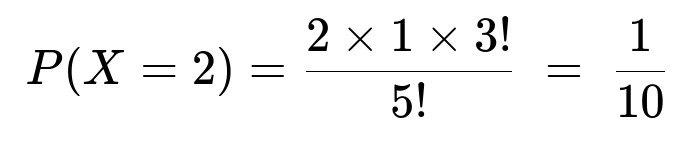
Case X = 2
We test only two batteries and find them both to be depleted. This event happens precisely when the two depleted batteries occupy the first two positions in the order.
The number of ways to place the 2 depleted batteries in positions 1 and 2 is 2! (i.e., those two depleted batteries can be permuted among the first two slots in 2! ways).
The remaining 3 good batteries can appear in any order in positions 3, 4, and 5 (that is 3! ways).
So there are 2! * 3! = 2 * 6 = 12 ways to have the two depleted in the first two positions. Out of 5! = 120 total permutations, the probability is:

Here:
2 is the number of ways to permute the two depleted batteries in the first two slots.
3! is the number of ways to order the remaining 3 good ones.
5! is the total number of permutations of all 5.
Case X = 3
We need exactly 3 tests if:
We do not see any depleted battery in the first two tests, but then find the first and second depleted ones on the third test, or
We see exactly one depleted battery in the first two tests, and then find the second depleted battery at the third test.
The short solution’s formula (often broken down by systematically counting how many permutations yield the second depleted battery exactly on the third test) gives:

The numerator structure reflects various ways to arrange where the depleted batteries can appear such that the third test reveals the second depleted battery.
Case X = 4
Finally, if we do not discover both depleted batteries in the first three tests, we will either discover it on the 4th test, or deduce it because it is the only possibility left. Numerically, since the probabilities must sum to 1 across the possible values of X (2, 3, and 4):

Hence, there is no scenario where we actually need a fifth test, because by the fourth test we either have already uncovered the second depleted battery explicitly, or we deduce it must be the untested one.
Putting It All Together
Thus, the probability mass function of X is:
P(X=2) = 1/10
P(X=3) = 3/10
P(X=4) = 6/10
These three probabilities sum to 1, indicating that these are the only possible stopping points in the procedure.
Follow-Up Questions
What if we insist on physically testing all 5 batteries, regardless of having deduced the second depleted battery earlier?
If we had a procedure where we continued testing until we physically see both depleted batteries (rather than stopping once we deduce the second is the last remaining one), then X would include the possibility of being 5. Specifically, in that scenario, if the second depleted battery happens to be the last battery in the sequence, you would actually test all 5. This problem’s statement clarifies we stop as soon as the two are identified or logically deduced, so 5 never occurs in the distribution.
Can we compute the expected value of X?
To find E[X] under the given stopping rule, we would compute:
E[X] = 2*(1/10) + 3*(3/10) + 4*(6/10)
Performing that:
2*(1/10) = 2/10 = 0.2 3*(3/10) = 9/10 = 0.9 4*(6/10) = 24/10 = 2.4
Adding them: 0.2 + 0.9 + 2.4 = 3.5
So E[X] = 3.5 tests on average.
How would we simulate this in Python?
Below is a straightforward way to simulate this process repeatedly, using random permutations of the five batteries, and checking how many tests are needed:
import random

def simulate_one_trial():
    # Represent depleted batteries as 'D' and good ones as 'G'
    batteries = ['D', 'D', 'G', 'G', 'G']
    random.shuffle(batteries)

    depleted_found = 0
    tests_performed = 0

    for i in range(5):
        tests_performed += 1
        if batteries[i] == 'D':
            depleted_found += 1
        # Stop as soon as the second depleted is found (or deduced)
        # Deduction scenario: if we've found 1 depleted in the first 4,
        # the 5th must be the other. So effectively, we stop at i=4 in that case.
        if depleted_found == 2:
            break
        if i == 3 and depleted_found < 2:
            # We know the last one must be depleted if we've only found 1 until now
            break
    return tests_performed

# Run many simulations
N = 1_000_000
counts = {2: 0, 3: 0, 4: 0}

for _ in range(N):
    x = simulate_one_trial()
    if x in counts:
        counts[x] += 1

# Estimate probabilities
for k in sorted(counts.keys()):
    print(k, counts[k] / N)
In this simulation:
We shuffle the list of five batteries (two depleted, three good).
We step through and check when we’ve identified the second depleted battery.
If by the 4th battery we’ve seen exactly one depleted, we stop too, because the 5th is deducible as depleted.
The empirical results from such a large simulation should approximate the theoretical probabilities 1/10, 3/10, and 6/10 for X=2, X=3, and X=4 respectively.
What are common pitfalls when dealing with such stop-on-deduction problems?
Forgetting Deduction: One typical mistake is to forget that, if there is only one battery left untested and exactly one depleted is still missing, you do not actually need to test the last battery. This can lead to an incorrect conclusion that X=5 is possible.
Miscounting Permutations: Another common pitfall is accidentally double-counting scenarios when enumerating permutations for X=3 or X=4.
Using Unconditional vs. Conditional Reasoning: Some try to compute P(X=2), P(X=3), P(X=4) purely by combinatorial arguments but forget to incorporate the logic that we stop as soon as we “know” we have found both depleted batteries.
These pitfalls highlight the importance of carefully enumerating or simulating the possible orders (or using correct conditional probability arguments) and keeping the stopping rule in mind at every step.
Below are additional follow-up questions
How might the distribution of X change if one of the two depleted batteries is more likely to appear earlier in the sequence due to prior knowledge or bias in the testing process?
In many real-world scenarios, batteries might not be shuffled uniformly. For instance, you could have prior knowledge or a physical arrangement that makes one depleted battery more likely to appear in an earlier test. This might happen if, say, the depleted batteries are physically labeled and you tend to pick from a certain side of the batch first.
Detailed Explanation
Non-uniform randomization: Instead of having 5! equally likely permutations, certain permutations might be more likely than others. This skews the probabilities for when you discover the depleted batteries.
Bayesian approach: If you know that “Battery 1” has a higher chance of being depleted than the others, you can integrate that prior probability into your calculations of P(X=k).
Potential pitfalls:
Incorrectly assuming uniform permutations when in reality the testing order is not truly random.
Overlooking physical or practical biases (like always testing the same side of a package first).
Edge case: If one battery is almost certainly depleted, the probability of discovering it early is very high. That could reduce the average number of tests needed because you effectively find the first depleted right away and only need to locate the second one.
What if the problem is modified so that you continue testing all batteries even after identifying two depleted ones, and you record X as the position of discovering the second depleted battery?
In this variation, instead of stopping immediately once you know the second depleted battery, you test all 5 anyway. The random variable X is the index of the test where the second depleted battery was first encountered in the testing sequence, but physically the testing continues to the end.
Detailed Explanation
Key difference: You do not terminate the testing process. The final test might be the 5th battery, but X is still the index where you first saw the second depleted battery. Hence X can be 2, 3, 4, or 5 in this scenario.
Pitfall:
Mixing up the idea of “position of discovery” vs. “position at which you stopped.” If you always test all batteries, you might still compute X incorrectly if you do not track the first moment you see the second depleted battery.
Edge case:
If the two depleted batteries happen to be in positions 1 and 5, you discover the second depleted battery only after going through all batteries, so X=5 in that scenario. However, you are still testing all 5, so physically you end with test number 5, but the random variable X is specifically the test number of the second depleted battery’s discovery.
Could the testing of a battery be prone to error, and if so, how would that affect the probabilities for X?
In practice, testing a battery might not always give a perfectly reliable result (false positives or false negatives). Suppose each test has a certain probability of incorrectly labeling a battery as depleted or good.
Detailed Explanation
Incorporating test errors: Let p be the probability that the test result is correct, and 1 - p be the probability that the test result is incorrect.
Implications:
You may not actually know for sure you found a depleted battery if the test can misclassify it.
Your stopping rule might be more complicated, because you might keep testing to confirm repeated observations.
Pitfalls:
Using the same approach as in the error-free scenario: The entire distribution for X changes, because even if you think you have found one depleted battery, it might have been a false positive.
Overconfidence: Stopping too early due to erroneous testing results.
Edge case: With a sufficiently low p (accuracy), you might effectively be unable to trust your test outcomes, requiring far more tests (or repeated tests of the same battery) to be confident in having identified both depleted batteries.
How does the reasoning change if there could be more than two depleted batteries in the set, say k depleted out of n total batteries?
A common generalization is that we have n batteries of which k are depleted, and we want the distribution for the number of tests until we identify all k depleted batteries (or deduce which ones they are).
Detailed Explanation
Generalization:
Let n be the total number of batteries.
Let k be the total number of depleted batteries.
The random variable X is the number of tests until we identify all k (or deduce any that remain untested are also depleted).
Pitfalls:
The combinatorial complexity grows quickly, because the possible permutations and the conditions under which you deduce the remaining depleted ones become more involved.
Failing to consider partial deduction steps, e.g., if you have found k-1 depleted batteries by test i, you might deduce the last one if there are only a small number of batteries left.
Edge cases:
k=1: Trivially, you only need up to n tests (but typically you stop when you find the single depleted battery).
k close to n: If almost every battery is depleted, you quickly discover many depleted ones, but you might also need more tests to confirm the last remaining battery’s state.
How might you handle a situation where you only learn the battery is “depleted or not” after a delay, rather than instantaneously?
In some real situations (imagine a hardware stress test), the result whether a battery is good or depleted might take time, so you cannot immediately know the result of test i before choosing battery i+1 to test.
Detailed Explanation
Delayed feedback: You might be forced to choose the next battery to test without knowing the result of the current or previous tests. This can lead to more complicated strategies rather than random permutations.
Possible approaches:
Sequential decision-making: If you must pick the next battery to test before having the result from the previous test, you might adopt a random approach or a scheduling approach to minimize total expected test time.
Pitfalls:
If you assume immediate feedback but it is actually delayed, you might incorrectly think you can stop early.
Over- or under-counting the number of tests, because you do not realize the results all come in at the end.
Edge case: If the test results are only available after you test all 5, the random variable X might not be well-defined as “the number of tests until you find the second depleted battery,” because you only know the outcomes at the end. You might instead define X differently, e.g., “the earliest index at which the second depleted battery was tested,” but you do not know that index until after all tests are done.
What if the testing order is chosen adaptively after each test result, instead of pre-randomizing all 5 batteries?
In many practical scenarios, you might choose which battery to test next based on the information gained so far (e.g., if a battery tested is found good, you might prefer to test a different battery next that you suspect is more likely depleted).
Detailed Explanation
Adaptive vs. non-adaptive testing: The original problem treats the order of testing as a single random permutation. In adaptive testing, after each test you decide the next battery to test based on prior results.
Pitfalls:
Trying to apply the same uniform-permutation arguments leads to inaccuracies because the sequence is no longer a simple random ordering—each step depends on outcomes from previous tests.
Edge cases:
If you discover one depleted battery very early, you might shift your strategy to specifically target the battery most suspect of also being depleted. This might lower E[X].
If you discover all good batteries quickly, you automatically deduce the last ones are depleted. The distribution can shift drastically compared to the uniform random approach.
If the problem extends to a situation where each test can be costly or time-consuming, is there an optimal strategy that minimizes the expected cost or time?
Rather than purely random testing, you might adopt a cost-minimizing approach. For example, some batteries might be quicker to test than others, or it might be more economical to test them in a certain order.
Detailed Explanation
Weighted or cost-based approach: Assign each battery a test cost or time. Then a testing sequence that minimizes expected total cost might differ from a random permutation.
Pitfalls:
Assuming equal cost: leads to the uniform random approach. Realistically, if some batteries are easier to test, you might test them first, which can alter the distribution for X or the expected cost.
Greedy vs. dynamic programming: A naive greedy approach (test the cheapest battery first) might not always be optimal if discovering a depleted battery early can drastically change your subsequent decisions.
Edge cases:
If testing one particular battery is virtually free, you might always do that test first, which shapes the distribution of X significantly. If it happens to be the depleted one, you reduce the overall search time drastically.
How would you apply these ideas to a real-world scenario like detecting defective items on an assembly line?
A typical industrial or manufacturing problem involves scanning items to detect which ones are defective. The analogy is that “depleted batteries” are “defective products,” and “good batteries” are “non-defective products.”
Detailed Explanation
Mapping to real-world:
“Batteries” become “units on the assembly line.”
“Depleted” becomes “defective.”
“Testing” is the quality check.
“X” is the test index at which you have found a certain number of defectives.
Pitfalls:
Real assembly lines might have items arriving continuously, so the concept of a fixed set of 5 is replaced by a flow or a stream of items.
There can be partial or delayed feedback from testing machines, or capacity constraints in how many items can be tested at once.
Edge cases:
If the defective items appear in clusters, the assumption of uniform permutations is invalid.
If some tests are destructive or irreversible, you might need to handle inventory constraints differently (e.g., once you test an item, it might be unusable or changed in some way).
How do you verify your combinatorial arguments, especially for more complex or larger setups?
Verification is crucial, especially when enumerating complicated sets of permutations and stopping rules. Typically, you can use either small-scale enumerations by code or large-scale Monte Carlo simulations.
Detailed Explanation
Exact enumeration: For small n, you can systematically list all permutations and count how many times X = k occurs. This ensures no mistakes in combinatorial reasoning.
Simulation: For larger n, enumerating all permutations might be infeasible, so you rely on random simulation of many trials.
Pitfalls:
Incorrectly implementing the stopping rule in simulation. For example, forgetting that you can deduce the second depleted battery when only one battery remains untested.
Failing to randomize properly. A flawed random number generator or shuffling algorithm can bias the simulated results.
Edge cases:
If the difference between the theoretical distribution and the simulated distribution is unexpectedly large, it often indicates a mistake either in the combinatorial logic or in the simulation code.
Best practice:
Compare theoretical results with simulation for small n.
Then rely on simulation for large n if necessary.
Could the concept of “negative testing” (i.e., testing to confirm a battery is good, not depleted) change the counting?
In some setups, you may be verifying a battery is good rather than directly looking for a depleted battery. Conceptually, though, it is quite similar—the event “battery is good” is just the complement of “battery is depleted.” But the order in which you interpret results could matter.
Detailed Explanation
Negative testing approach:
Instead of “We are searching for the depleted ones,” your mindset might be “We are searching for evidence that a battery is still good.”
However, from a probability perspective, it’s just the complement—still 2 are not good, 3 are good.
Pitfalls:
If your test is specifically tuned to detect ‘goodness’ rather than ‘badness,’ false negatives or positives might occur differently from the standard assumption.
You might inadvertently double-count or mislabel tests if the test is more sensitive to one condition than the other.
Edge cases:
A test that can confirm a good battery with near 100% accuracy but can only detect depletion with lesser accuracy. This imbalance can alter your stopping strategy if you rely more heavily on confirming a battery is good.
If multiple testers operate in parallel, does it affect the distribution of X?
Imagine you have two or more testers that can test batteries simultaneously. This scenario changes the timing of when you discover depleted batteries.
Detailed Explanation
Parallel testing:
You might test 2 or more batteries in each round. The random variable X might represent the total number tested up to the point at which you have discovered both depleted batteries.
Pitfalls:
The outcomes from multiple tests per round might arrive at different times or all at once, so you have to carefully define how you “stop” and what X represents (the number of rounds vs. the total number of individual tests used).
Edge case:
If you have enough testers to test all 5 batteries at once, you effectively discover both depleted batteries after a single round. The distribution collapses to X=1 round in that interpretation. But if X is the “index of the test,” it might need redefinition.
In a practical setting, how can partial recharging or borderline depletion complicate the model?
You might have borderline batteries that sometimes pass initial tests but fail under heavier load. The concept of “depleted vs. good” can become fuzzy.
Detailed Explanation
Gray area: A battery might fail under certain conditions but pass under others, so labeling it “fully depleted” might be context-dependent.
Pitfalls:
Using a binary model (depleted vs. good) when reality is more nuanced can lead to inaccurate estimates of how many tests you truly need.
You might retest borderline batteries under more stringent conditions, changing the distribution of how quickly you discover them as “truly depleted.”
Edge cases:
A battery that behaves “good” in the first test but fails in a retest. This can upend the logic that once you label it good, you never re-check it. In reality, you might need repeated tests to confirm a borderline battery’s status.