
ML Interview Q Series: Probability of More Heads in n+1 vs n Fair Coin Flips Using Symmetry.

Browse all the Probability Interview Questions here.
17. A and B are playing a game where A has n+1 coins, B has n coins, and they each flip all of their coins. What is the probability that A will have more heads than B?
A thorough way to see why the final answer is one-half centers on a symmetry argument: since both players’ coins are fair, and A has exactly one extra coin, that extra coin essentially serves as a “tiebreaker.” More rigorously, we show below that the probability of A having strictly more heads than B is 1/2.
Explanation of the Key Idea
One way to see this is to note that any outcome for the first n coins of A can be matched with an outcome for B’s n coins. Now, consider A’s extra coin. If the other n coins of A and B’s n coins produce the same number of heads, then the extra coin of A determines whether A’s total heads exceed B’s. If A’s extra coin is Heads, then A surpasses B; if it is Tails, then they stay tied (if the rest were tied). Meanwhile, in cases where the first n coins of A already have more heads than B (or vice versa), that outcome is also balanced by corresponding outcomes in which B has more heads than A, by symmetry across fair coin flips. Putting all this together shows that overall, the probability of A having strictly more heads than B is 1/2.
More Formal Probability Argument
Let H_A be the random variable for the number of heads A gets from all n+1 flips, and H_B be the random variable for the number of heads B gets from n flips. Both H_A and H_B are binomially distributed, but H_A ~ Binomial(n+1, 1/2) while H_B ~ Binomial(n, 1/2). We want

We can write:

By symmetry arguments on fair coins (and also combinatorial reflections), we get:
Then it follows that:

so

We also note that if A has exactly one more coin than B, the probability of a strict tie in the total number of heads is the probability that the extra coin offsets the difference in heads from the other n coins. One can show through combinatorial sums or other arguments that this leads precisely to

This holds for all n ≥ 0. For instance, if n=0, A flips 1 coin, B flips 0 coins, and the probability that A gets more heads is simply the probability that A’s single coin shows heads, i.e. 1/2. The same 1/2 result holds for general n.
Detailed Intuitive Explanation
One particularly direct intuition is to imagine labeling A’s flips as Flip 1, Flip 2, …, Flip n+1, and labeling B’s flips as Flip 1, Flip 2, …, Flip n. Pair up Flip 1 of A with Flip 1 of B, Flip 2 of A with Flip 2 of B, and so on, up to Flip n of A with Flip n of B. Now all those pairs can produce the same or differing numbers of heads. Finally, A still has that extra (n+1)-th flip. Because each coin is fair, whenever the first n pairs collectively favor B, there is a correspondingly mirrored scenario (by flipping outcomes) where they favor A. The extra coin ends up being the deciding factor half the time in the overall sense. Thus, the probability that A finishes with strictly more heads is 1/2.
Example for Small n
When n=1, A has 2 coins and B has 1 coin. Enumerating all outcomes:
B can get 0 heads (probability 1/2) or 1 head (probability 1/2). A can get 0 heads (1/4), 1 head (1/2), or 2 heads (1/4).
Counting the scenarios shows that the total probability of H_A > H_B is 1/2, which matches the general reasoning above.
Simulation Example in Python
Below is a straightforward simulation that illustrates this concept for large n. This is just to confirm the theoretical result in practice.
import random
import numpy as np

def simulate_probability(num_trials=10_000_00, n=10):
    count_A_wins = 0
    for _ in range(num_trials):
        # A flips n+1 coins
        A_heads = sum(random.randint(0, 1) for __ in range(n+1))
        # B flips n coins
        B_heads = sum(random.randint(0, 1) for __ in range(n))

        if A_heads > B_heads:
            count_A_wins += 1

    return count_A_wins / num_trials

prob_estimate = simulate_probability()
print(prob_estimate)  # Should be very close to 0.5
In a large number of trials, the outcome of “A has more heads” will hover near 0.5, illustrating the 1/2 probability.
Practical Follow-up Considerations
It is common to wonder if this result changes if coins are weighted (not fair) or if different players use different coin biases. The entire 1/2 result strictly depends on all coins being fair (probability 1/2 for heads). If coin biases change, the probability needs to be computed through generalized binomial sums.
Below are further follow-up questions with full, detailed answers.
What if the coins are not fair?
If each coin for A and B has some bias p for landing heads (the same bias for all coins), then A’s total heads, H_A, follows a Binomial(n+1, p) distribution, while B’s total heads, H_B, follows a Binomial(n, p) distribution. In that case, symmetry breaks down, and we can no longer say that the probability of A having more heads is 1/2.
More specifically, we would compute:

where
and
1[⋅]
is the indicator function that is 1 if the condition is true and 0 otherwise. This sum can be computed directly if n is not too large. We will find that, generally, this probability is greater than 1/2 if p > 1/2 (A has an advantage from both having an extra coin and the coin itself favoring heads more than tails) and less than 1/2 if p < 1/2 (the extra coin helps, but each individual coin is biased to land tails more often).
Could you show a purely combinatorial argument for the fair-coin case?
Yes. One combinatorial approach goes as follows:
Consider all possible outcomes of flipping (n+1) + n = 2n+1 fair coins. There are

equally likely global outcomes. Now define two outcomes:
• One outcome is (a_1, …, a_{n+1}) for A and (b_1, …, b_n) for B, with a_i, b_j ∈ {H, T}. • Another outcome is (b_1, …, b_n) for B and (a_1, …, a_{n+1}) for A, but shift the indexing or consider a reflection that pairs them up systematically.
Because the total number of coins is odd (2n+1), exactly half of all possible ways to distribute heads and tails across those 2n+1 flips will produce a strictly greater number of heads for A, except for those cases where A and B end up tying. By carefully pairing up outcomes in a reflection sense, one can show that all of them group into either “A has more heads” or “B has more heads” pairs, with the leftover possibility being ties. Because an extra coin for A systematically shifts that reflection argument in A’s favor by exactly one flip, we get P(A > B) = 1/2.
How would you handle large n in practice if you wanted to confirm this probability?
If n is large, a common practical approach is to rely on the normal approximation or a direct simulation. For large n, the binomial distributions can be approximated by Gaussians:
H_A ~ Binomial(n+1, 1/2) can be approximated by a Normal(mean = (n+1)/2, variance = (n+1)/4).
H_B ~ Binomial(n, 1/2) can be approximated by a Normal(mean = n/2, variance = n/4).
We would then approximate

where Z is a standard normal random variable. The difference in means is –1/2, and the variance of the difference is ((n+1)/4 + n/4) = (2n+1)/4. This transforms to:

Because that expression goes to 0 for the argument in the numerator if we do direct expansions, a more rigorous pairing argument or direct simulation is easier. In any case, we can do a Monte Carlo simulation (as shown earlier) in code to get an empirical measure. That numeric simulation robustly shows P(A has more heads) → 1/2.
What if we instead ask: what is the probability that A gets exactly one more head than B?
That is a different question than “strictly more heads.” To calculate

for k = 0, 1, …, n. Summing over all possible k,
In simplified form, that is exactly the probability that A’s total is exactly 1 greater than B’s total. It is not 1/2. In fact, that number is related to the distribution of the difference H_A – H_B. However, once we sum up all ways in which A’s total can exceed B’s by any positive integer, that entire probability sums to 1/2.
Are there any intuitive pitfalls or tricky details?
One subtlety is not to confuse “A has more heads than B” with “A has more heads than or equal to B.” The question asks strictly more. The presence of the (n+1)-th coin for A ensures the tie scenario does not split the 1/2–1/2 symmetry in the usual way. Another pitfall is mixing up the distribution of differences for binomial random variables versus the distribution for each variable itself. One must be careful about how reflection or pairing arguments are constructed, but the key is that with fair coins, each outcome has a symmetrical counterpart.
Another pitfall is to overlook the assumption of fairness: the entire 1/2 result breaks down if the coins are biased or if they differ between A and B. Also, if there were multiple extra coins on A’s side or if the coin counts differ by more than 1, the probability obviously differs from 1/2 in general.
All the above clarifications confirm that, for fair coins, the probability that A, with n+1 coins, ends up with more heads than B, with n coins, is 1/2. There is a simple tie-breaking logic and a more rigorous combinatorial or distribution-based reasoning all leading to the same 1/2 conclusion.
Below are additional follow-up questions
What if there is a chance a coin could land on its edge instead of heads or tails?
If we allow a small probability that a coin lands on its edge (and we treat that edge outcome as neither heads nor tails), the setup changes fundamentally. Let p = probability of heads, q = probability of tails, and r = probability of landing on edge, where p + q + r = 1.
To address “more heads” with an edge possibility, each coin flip now has three possible outcomes. Let H_A be the number of heads for player A, and H_B be the number of heads for player B. Suppose A flips n+1 coins and B flips n coins. The distribution of heads for A (H_A) and B (H_B) are now multinomially influenced but can be viewed as:
• H_A still counts how many times an A coin lands heads among the n+1 coins, each with probability p for heads. • The difference from a standard binomial is that the total probability mass for heads on each coin is p, for tails is q, and for edge is r, rather than a 1/2–1/2 split.
We want to find P(H_A > H_B). Each coin for A or B can produce heads with probability p, or not-heads (tails or edge) with probability q+r = 1 – p.
Key Points and Reasoning: • If r = 0, we revert to the biased or fair coin scenario. • If r > 0, we interpret that any non-head outcome (tail or edge) does not increment the head count. This effectively preserves the “heads vs. not-heads” viewpoint but with heads happening with probability p < 1. • Hence H_A ~ Binomial(n+1, p) (assuming each coin’s edge outcome is just lumped into “no head”). Likewise, H_B ~ Binomial(n, p).
Therefore, even if a coin can land on its edge, the probability of “head” is still p, and “not-head” is (1 – p). We ignore the distinction between tails and edges in terms of counting heads; both are simply not-head. We then revert to computing:
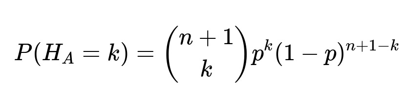
P(H_A > H_B) = sum_{k=0}^{n+1} sum_{j=0}^{n} [P(H_A = k) × P(H_B = j) × 1(k > j)],
where P(H_A = k) = C(n+1, k) p^k (1 – p)^(n+1 – k), P(H_B = j) = C(n, j) p^j (1 – p)^(n – j).
If p = 1/2 and r = 0, we get the 1/2 probability for A > B. If r > 0 but p still equals 1/2 of (p + q)—in other words, if the coin still “heads” half the time it is not on edge—this interpretation might be more subtle. Strictly speaking, the probability that a flip is heads is p (not necessarily 1/2). The final result can only revert to 1/2 if p = 1/2. Otherwise, it is a biased coin scenario with an extra “edge” category that does not contribute to heads.
Pitfall to Watch Out For: A common oversight is to assume the presence of an edge outcome changes the fundamental symmetry for heads vs. tails. In reality, from the standpoint of counting only heads, every edge or tail is effectively the same in that it’s not a head. So the net effect is that each coin has probability p for heads, and (1 – p) for not-head. That factor p could still be 1/2 if the design is such that heads and tails+edge are equally likely overall, but typically p would be smaller than 1/2 if edge is possible.
How does the probability change if the coin flips are correlated rather than independent?
If A’s (n+1) flips and B’s n flips are not independent, the calculation can get complicated because the typical binomial assumptions break down. For example, imagine a scenario where if a certain coin for A comes up heads, it increases (or decreases) the chance that a certain coin for B will also come up heads, or vice versa.
Key Considerations for Correlation: • If correlation is positive (i.e., an event that A gets many heads makes it more likely that B also gets more heads), it could influence P(H_A > H_B) in a non-trivial way. Intuitively, if both sets of flips “move together,” we might expect more tie scenarios or less separation in the counts of heads. • If correlation is negative, then A having more heads might systematically make B have fewer heads, which could lead to a probability that differs (often larger) than 1/2 when n+1 vs. n coins are used.
No Simple Closed-Form: There is typically no simple closed-form expression for P(H_A > H_B) under correlated flips. One would need a joint probability model for the entire set of flips. For instance, if we specify a correlation coefficient ρ for pairs of Bernoulli random variables, we are effectively specifying a more general distribution (e.g., using a copula or some parametric form). In that setting, we would:
Define the joint distribution of the 2n+1 Bernoulli random variables (A’s n+1 plus B’s n).
Sum or integrate over that joint distribution the event {H_A > H_B}.
In practice, one might resort to simulation:
Generate correlated Bernoulli variables (e.g., via underlying correlated Gaussian “latent” variables with a threshold transform)
Count how often H_A > H_B.
Pitfalls: • Even a small correlation can shift probabilities away from 1/2. • If the correlation structure is unknown, a naive assumption of independence can produce incorrect conclusions. • Real-world coin flips are typically assumed independent, but in certain mechanical or contrived setups, correlation might arise (e.g., if the same physical “toss” of multiple coins influences their outcomes in a structured way).
How does the result change if A and B’s coins differ in number by more than 1?
So far, the known result of P(A > B) = 1/2 is specific to the situation where A has n+1 fair coins and B has n fair coins. If we generalize:
• Let A have m coins and B have n coins, both fair. • Then H_A ~ Binomial(m, 1/2) and H_B ~ Binomial(n, 1/2).
We want P(H_A > H_B). There is no simple universal formula that always equals 1/2 unless m = n+1. One can find general expressions:
P(H_A > H_B) = sum_{k=0}^{m} sum_{j=0}^{n} [P(H_A = k) × P(H_B = j) × 1(k > j)].
Even for m = n + 2, we lose the neat symmetry argument that yields 1/2. Usually, if m > n, P(H_A > H_B) will exceed 1/2, but the exact value is not trivially 1/2 anymore. As m – n grows, the probability that A ends up with more heads grows above 1/2.
Example: • If A has 2 coins and B has 1 coin (that is actually the n=1 scenario, so n+1=2, we do get 1/2). • If A has 3 coins and B has 1 coin, we can do a direct enumeration or a binomial-based sum. In that scenario, the probability that A has more heads is definitely greater than 1/2 because the advantage is more than just a single extra coin.
Pitfall: • A common mistake is to assume that for any difference in coin counts, the probability that the player with more coins has strictly more heads is always 1/2. That is not correct. The 1/2 result depends heavily on the difference in coin counts being exactly 1 (and the coins being fair).
What if the winner is determined by “at least as many heads” instead of strictly more heads?
If the game is changed so that A “wins” or “meets the condition” whenever H_A ≥ H_B, that is a different probability:
P(H_A ≥ H_B) = P(H_A > H_B) + P(H_A = H_B).
From the known result P(H_A > H_B) = 1/2 for A having n+1 coins (and B having n coins) with fair flips, we need to add P(H_A = H_B). We can find P(H_A = H_B) by enumerating or summing:
P(H_A = H_B) = sum_{k=0}^{n} [P(H_A = k) × P(H_B = k)], where H_A ~ Binomial(n+1, 1/2), H_B ~ Binomial(n, 1/2).
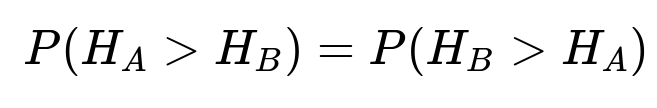
A simpler approach: From the symmetry argument:
1 = P(H_A > H_B) + P(H_A < H_B) + P(H_A = H_B). But P(H_A > H_B) = P(H_B > H_A). So: 1 = 2 P(H_A > H_B) + P(H_A = H_B). Given P(H_A > H_B) = 1/2, we get P(H_A = H_B) = 1 – 2 × (1/2) = 0. But that would suggest zero probability for H_A = H_B, which seems contradictory until we notice that n+1 + n is an odd total of coins. The total number of heads across all coins can be from 0 up to 2n+1. Because the total number of coins is odd, the number of heads across all flips cannot be split equally between A and B unless A’s extra coin comes out tails (making them effectively have n coins that produce heads among the same total?). Actually, let’s clarify carefully:
In the typical pairing argument, it might appear that P(H_A = H_B) = 0 for the scenario of n+1 vs. n fair coins. Indeed, for small n, we can check explicitly:
If n=0, B has 0 coins, H_B=0. A has 1 coin, H_A≥0. Probability(A = B) means A has 0 heads, so that is a 1/2 probability. Actually that’s 1/2 for H_A=0. That implies a tie of 0 heads each. So it’s not 0.
For n=1, A flips 2 coins, B flips 1 coin. The probability that H_A = H_B can be enumerated: both get 0 heads if A gets 0 heads and B gets 0 heads. Probability = (1/4)(1/2)=1/8. Also, they both get 1 head if A gets exactly 1 and B gets exactly 1. That’s (1/2)(1/2)=1/4. Summing, that’s 3/8, not 0.
Hence, for general n, P(H_A = H_B) is definitely not 0. What is correct is the result:
P(H_A > H_B) = 1/2 implies P(H_A < H_B) = 1/2 – P(H_A = H_B).
The symmetry argument that yields P(H_A > H_B) = 1/2 does not forcibly require P(H_A = H_B) to be 0. Instead, it enforces that among all outcomes that are not ties, half favor A and half favor B. This is a subtlety: the probability of a tie is the same from both vantage points, so the non-tie portion of the outcome space is split evenly.
Hence, if we ask for P(H_A ≥ H_B), that is:
P(H_A ≥ H_B) = 1/2 + P(H_A = H_B).
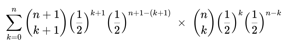
We need to compute P(H_A = H_B). For fair coins, it’s not trivial to express in a single closed form, but we can do:
P(H_A = H_B) = sum_{k=0}^{n} [C(n+1, k) (1/2)^{n+1} × C(n, k) (1/2)^{n}].
So the final probability is strictly greater than 1/2.
Pitfall: • The notion that “A always has at least as many heads as B half the time” is incorrect once we allow equality. The probability of “A has at least as many heads” is strictly greater than 1/2 because ties exist.
What if each player can choose how to allocate some resource across their coin flips (e.g., flipping speed or method) to influence heads?
While in a purely theoretical, idealized coin flip scenario each coin flip is fair with no advantage from technique, a real-world or strategic scenario might allow players to attempt to influence the distribution of heads by certain flipping strategies (such as spin velocity, angle, or distribution of tosses). This is more of a practical or psychological question, but can be asked in interviews to see if the candidate recognizes that physical coin flips might not always be perfectly fair or i.i.d.
Reasoning on Possible Influences: • If a coin is physically biased by the flipping technique, the probability of heads can deviate from 1/2. • If B can produce a distribution that yields near 50% heads for B but somehow forces A’s coin outcomes to deviate or be more random, or vice versa, that might affect the overall probabilities. • Typically, we assume each coin flip is identically distributed and independent. Real-world physical effects can break these assumptions.
Potential Pitfalls: • Overlooking that real coin flips are not necessarily pure Bernoulli(1/2). The question “What if A is better at flipping coins?” might push the probability away from 1/2. • There may be partial correlation introduced if both players share the same environment, like wind or a table surface that influences bounce and final resting state.
Conclusion Under This Twist: The original theoretical result P(H_A > H_B) = 1/2 only holds exactly if each coin is fair, identically distributed, and the flips are independent. If these conditions are violated by different flipping “techniques,” you must model or measure the new distribution or correlation for each coin flip to calculate the correct probability.
What happens if the players keep flipping until they each decide to “stop,” with A allowed n+1 total stops and B n total stops?
This question drastically alters the nature of the problem. Instead of a simple one-shot scenario where all coins are flipped simultaneously, we imagine a sequential or dynamic game where each player can choose to “bank” some number of heads or skip flips. A might have n+1 attempts to accumulate heads, while B has n attempts.
Key Observations: • This becomes akin to an optimal stopping or gambler’s ruin–style problem. • The random variables for heads in each flip are no longer purely binomial if each player tries to time or choose favorable flips.
If the flips remain fair and independent across attempts, and if the players have no predictive power about whether the next flip will be heads or tails, then the advantage from having an extra flip (for A) is simply more chances to accumulate heads. The exact probability that A ends with more heads would still be greater than 1/2 if A actually uses that additional flip.
Pitfalls: • The question’s constraints—“they each flip all of their coins”—are replaced by a scenario with strategy. That changes the distribution from binomial to something else. • If each player can see partial results and decide to keep flipping or not, the game theory becomes more complex, but typically having an extra coin flip is still an advantage.
Thus, the original simplicity of P(H_A > H_B) = 1/2 relies on a straightforward, simultaneous flipping scenario. With sequential or optional flipping, the entire model changes.
Could the same 1/2 argument hold if A’s coin flips are performed first, and B decides to flip after seeing A’s results?
If B is allowed to see A’s outcomes in advance, B gains a crucial advantage—knowledge of how many heads A got—before flipping. Then B can tailor decisions (if B had any strategic choice) or just mentally note the number to see if B can exceed it. Even if B must still flip all n coins, seeing A’s results does not change the coin distribution directly, but it changes B’s expected chance to surpass A if B can do something strategic.
If the flips remain purely fair and B has no control (i.e., must flip all coins anyway), the knowledge alone does not change the distribution of B’s heads. The underlying probability P(H_A > H_B) remains 1/2 from a purely mathematical standpoint if all flips are still fair and the number of flips is n+1 for A, n for B. The only difference is that B psychologically knows in advance what they must beat.
Pitfalls: • Confusing knowledge with control. Observing A’s outcomes in advance does not help if B cannot alter the coin’s probability of landing heads. • If B is given a strategic mechanism (like re-flipping tails, or changing a coin bias after seeing A’s result), it breaks the original assumption and yields a different game.
Hence, in a straightforward scenario where B just sees A’s results but flips the same n fair coins (with no further strategic advantage), the probability is still 1/2 that A ends with more heads. The knowledge does not shift the distribution of heads for B.
What if the notion of “winning” is replaced by a margin threshold, such as “A wins if A has at least 2 more heads than B”?
If we define a new event: “A has at least d more heads than B,” i.e. H_A ≥ H_B + d, this is a stricter condition than simply having more heads (which is d=1). In that case:
P(H_A ≥ H_B + d) = sum_{k=d}^{(n+1)} sum_{j=0}^{n} [P(H_A = k) × P(H_B = j) × 1(k ≥ j + d)].
For d=1, we get the usual “strictly more heads” scenario. For d=2 or higher, the probability is necessarily smaller than the probability that H_A > H_B. Because the advantage of one extra coin helps, but sometimes that single extra coin yields only a 1-head advantage or none, especially if it lands tails.
Intuition: • For d=2, A must surpass B by at least 2 heads. Even though A has an extra coin, there is a decent chance the margin remains 0 or 1 head. That portion of the outcome space no longer counts as A “winning.” • Typically, the probability that A has at least 2 more heads than B is less than 1/2 for large n, though it grows with n in interesting ways.
Pitfall: • Overgeneralizing the 1/2 result. That 1/2 result specifically applies to “strictly more heads.” For any margin d>1, the probability will generally be below 1/2.
What is the probability distribution of the difference in heads, D = H_A – H_B, and does that help confirm the result?
Defining D = H_A – H_B: • H_A ~ Binomial(n+1, 1/2), H_B ~ Binomial(n, 1/2). • The difference D can range from -(n) up to n+1.
One might attempt to compute P(D = d) for d in that range. A direct formula for the difference of two binomial random variables is:
P(D = d) = sum_{k} P(H_A = k) × P(H_B = k – d),
where the sum is taken over any k such that k – d is a valid range for B’s heads. If we specifically focus on P(D > 0), that is exactly P(H_A > H_B).
How This Confirms the 1/2 Result: If we sum P(D = d) over d > 0, we get the probability that A has more heads. When we carefully carry out that sum or apply symmetry arguments, we arrive at 1/2. The advantage of having one extra coin ensures that, among all possible outcomes, half of the non-tie outcomes favor A.
Pitfall: • Overlooking the fact that the difference distribution for two binomials that are not the same size is not symmetric around 0. Indeed, if both had n coins (the same number), P(H_A – H_B = 0) could be substantial, and the distribution might center on 0. But with n+1 vs. n coins, the distribution of D is shifted. Nonetheless, the event {D > 0} has probability 1/2 (for fair coins), once we account for the possibility of ties.
What happens if we consider an “infinite coin” limiting argument?
One might consider taking n → ∞, letting A have n+1 coins and B have n coins, and then examine the fraction of heads. In that limit, the fraction of heads for A is H_A / (n+1) and for B is H_B / n. Each fraction tends (by the Law of Large Numbers) to 1/2. On average, for very large n, H_A is roughly (n+1)/2 and H_B is roughly n/2. The difference in expected values is 1/2, but that is not enough to guarantee A always beats B. The question remains about the distribution around those means.
Using a Central Limit Theorem argument: • H_A ~ ~N((n+1)/2, (n+1)/4) for large n. • H_B ~ ~N(n/2, n/4). • The difference H_A – H_B then has mean (n+1)/2 – n/2 = 1/2, variance (n+1)/4 + n/4 = (2n+1)/4, so standard deviation ~ √(2n+1)/2.
As n grows large, the difference’s distribution spreads out on a scale of roughly √n, but the mean difference is 1/2. The fraction of the time that this difference is greater than 0 is effectively the fraction that a N(0.5, (2n+1)/4) random variable is above 0. For large n, that fraction converges to 1/2 because 0.5 is negligible compared to the ~√n standard deviation. We can confirm that, even in the limit, the probability that A’s difference is above 0 remains 1/2.
Pitfall: • Mistakenly assuming that since the difference in means is 1/2, that automatically means the probability is near 1 for large n. That is not correct: the standard deviation scales with √n, so the effect of a mere 0.5 difference in means is negligible at large n. We still get 1/2.
If we track not just who gets more heads, but also how many total flips landed heads overall, does that change the conclusion about P(A > B)?
Sometimes an interviewer might extend the question: “We also want to know the distribution of the total heads T = H_A + H_B across all 2n+1 coins. Does analyzing T help us figure out the probability that A gets more heads?”
• The total T can range from 0 to 2n+1. • For each fixed T = t, the number of ways to split t heads among A’s n+1 coins and B’s n coins is combinatorial. • Summing over all possible t, we can ask: “Given T = t, what is the probability that H_A > H_B?”
We still get the same final answer of 1/2 for the unconditional probability that H_A > H_B, because each total t occurs with some binomial coefficient weighting, and within each t we see how it can split between A and B. The symmetrical reflection argument about how the t heads might be distributed still leads to half of the non-tie splits favoring A.
Pitfalls: • Attempting to use T to “simplify” might actually complicate the analysis if not done carefully. The event “A gets more heads than B” is about a partition of T heads, but T itself is random. Summing over T requires a conditional approach that can be more cumbersome than a direct binomial or symmetry argument. • Confusing the distribution of T with the distribution of H_A alone can lead to mistakes in evaluating the conditional probabilities.
In the end, analyzing T is an alternate combinatorial method, but does not alter the fundamental 1/2 conclusion.
Could the coins be multi-sided objects that produce “heads” if they land on one of multiple faces?
Another interesting variation is if each “coin” is replaced by an m-sided die, with some subset of faces counted as “heads.” For instance, suppose an m-sided object has 1 face labeled “heads” and (m–1) faces labeled “not-heads,” each equally likely. Then the probability of “heads” in a single flip is 1/m, effectively a biased Bernoulli. A has n+1 flips, B has n flips.
Everything then follows the same logic as a binomial distribution with parameter p = 1/m. Specifically: • H_A ~ Binomial(n+1, 1/m). • H_B ~ Binomial(n, 1/m).
The question of P(H_A > H_B) requires summing or symmetrical reflection arguments for a biased coin scenario (p = 1/m). If m=2, that’s just the standard fair coin case with probability 1/2 of heads. Otherwise, P(H_A > H_B) will differ from 1/2. Typically, if p < 1/2 (like 1/m for m>2), A’s extra coin helps, but not necessarily to the point that P(H_A > H_B) is exactly 1/2.
Pitfall: • Conflating the multiple faces with a 1/2 chance for heads. If there is only one “winning” face on an m-sided object, the probability is 1/m, not 1/2. The extra coin can still be an advantage, but the final probability that A surpasses B is not guaranteed to be 1/2.
Could we interpret the result with a random walk perspective?
Sometimes these coin-flip problems can be mapped to random walks or Markov chains. Suppose we define a 1D walk that increments by +1 each time A gets a head and increments by –1 each time B gets a head. If each has the same number of flips, we might track the distribution of the walk. However, when A has one extra flip, the random walk perspective can still apply but we have an imbalance in the total steps taken by “A vs. B.”
In a typical gambler’s ruin or random walk interpretation: • Each step is either “A’s head” or “B’s head.” • If all coins were aggregated into a single sequence of 2n+1 flips, we might parse out which flips belong to A vs. B.
Yet, the result P(H_A > H_B) = 1/2 emerges more transparently from direct binomial or symmetry arguments rather than a standard gambler’s ruin approach. The random walk analogy can become confusing if we are not careful about how steps are counted for each player.
Pitfalls: • In standard gambler’s ruin problems, the total number of steps for each side is typically the same, or the stepping is turn-by-turn. Here, A simply has one more coin to flip in total, which is not the typical random walk format. • If we try to combine flips into a single sequence, we must be precise in how we define “move for A” vs. “move for B.”
Hence, while a random walk perspective can sometimes help with intuition (e.g., about the difference in heads), it is not as straightforward here as the direct binomial approach or the pairing argument.
What if we track the time or order in which heads appear? Does that affect the final probability?
Another variation is: “Does the order in which A or B obtains heads matter to the final outcome?” For instance, if we record which flip each player got heads on, does that change the probability that A ends with more heads?
Under the standard assumption (all flips are fair and performed in a single batch or independently): • The order in which heads appear does not change the final count of heads for each player. • The probability question “Does A have more heads than B at the end?” depends only on the total number of heads, not on the sequence of flips.
If we introduced a rule that “the game ends as soon as one player has more heads than the other,” that changes the dynamic. But that is not the question asked.
Therefore, order is immaterial for the original scenario. The probability that A finishes with more heads is unaffected by whether we track the order in which heads appear.
Pitfall: • Assuming that if B gets an early lead in partial flips, that implies B has a higher probability of finishing with more heads. That is a sequential viewpoint. If we still flip all coins, the final distribution remains unchanged by intermediate states. The standard problem is about the final count.
Could we recast the problem in terms of “one group of n+1 coins vs. another group of n coins” with a shared sample space, and does that help?
Yes. Another vantage point is to imagine that all 2n+1 coins are flipped at once. Then we randomly assign n+1 of those coins to A and the remaining n coins to B. Because the coins are fair and identical, every assignment of coins is equally likely. Now, we ask: “What is the probability that the group of n+1 coins assigned to A shows more heads than the group of n coins assigned to B?”
A symmetrical reflection argument can be constructed by pairing each assignment with its “complementary assignment.” Precisely half of the ways to split the coins into an (n+1)-subset vs. an n-subset will result in A’s subset having more heads. The remainder of the ways will result in B’s subset having more heads, except for the smaller fraction that ties. But by carefully analyzing the combinatorial structure, we still get P(H_A > H_B) = 1/2 for fair coins.
Pitfall: • Confusing the random assignment perspective with the direct flipping perspective. In truth, they are consistent because each coin is fair. But one must keep track carefully of how the subsets are chosen and confirm that “A’s subset has strictly more heads” lines up with the original scenario.
If the result for n+1 vs. n coins is exactly 1/2, could there be any rounding or numerical issues in computational implementations for large n?
When implementing the probability in software (e.g., summations of binomial PMFs), for large n, floating-point approximations can introduce small numerical errors. For instance, summing:
P(H_A = k) × P(H_B = j) over k > j
might yield something very close to 0.5 but not exactly. The result might come out as 0.4999999998 or 0.5000000012, etc., depending on the floating-point representation.
Key Observations: • Theoretically, it is exactly 1/2. • Numerically, simulations and direct binomial sums for large n are subject to floating-point errors, but the limit is still 0.5. • Using exact rational arithmetic or specialized libraries for binomial coefficients can yield the precise fraction 1/2 if carefully computed.
Pitfall: • Concluding from a small floating-point discrepancy that the probability is not 1/2. In practical large-scale computing, always check for numerical stability.
Does the result hold if we interpret “coin flips” as some generic 0/1 process that sums to n+1 vs. n?
Yes. The essence of the result does not rely on a physical coin but on any set of i.i.d. Bernoulli(1/2) variables. Whether these come from a random bit generator, a quantum measurement, or a classical coin, the distribution is the same. The total of n+1 i.i.d. Bernoulli(1/2) trials is Binomial(n+1, 1/2). Similarly for B with n trials.
As soon as we confirm: • Two sets of i.i.d. Bernoulli(1/2) variables, one set of size n+1, the other of size n, and • All trials are independent across sets,
then P(H_A > H_B) = 1/2. That is a fundamental property of Bernoulli(1/2) processes with a one-trial difference.
Pitfall: • Overthinking the “coin” aspect. If we replace flips with any independent “Bernoulli(1/2)” trials, the mathematics remains the same. The real question is the independence and fairness (p=1/2).
Is there a direct combinatorial identity that shows P(H_A > H_B) = 1/2?
Yes, there is a known combinatorial identity:
Sum_{k=0}^{n+1} Sum_{j=0}^{n} [C(n+1, k) C(n, j) (1/2)^(n+1) (1/2)^n * 1(k > j)] = 1/2.
A well-known approach uses:
C(n+1, k) C(n, j) = C(2n+1, k+j) × some ratio factor,
plus an argument that exactly half of the subsets of an odd number of elements contain more elements in one subset than the other, once we exclude ties. Another direct proof uses reflection: for each way to have H_A = k, H_B = j, we can reflect heads to tails and tails to heads or swap positions in a carefully defined manner. That combinatorial reflection shows the event (H_A > H_B) is in bijection with (H_B > H_A), forcing them to have equal probability.
Pitfall: • Missing the detail that the total number of coins is 2n+1, which is odd, so the combinatorial reflection or pairing works out neatly. If the total were even, the argument changes.
Does this 1/2 probability depend on n being finite?
Yes, but only in the sense that the argument is valid for all finite n ≥ 0. One can also consider the limit n → ∞. The probability remains 1/2 in that limit, as argued by the Central Limit Theorem approach or direct combinatorial reasoning. For each finite n, it is exactly 1/2; as n grows, it stays 1/2.
Pitfalls: • Mixing up the limit n → ∞ with some large-n approximation that might incorrectly yield a probability near or far from 1/2. The correct approach still yields 1/2 in the limit. • Overlooking that if n is extremely large but the coin is truly fair, the advantage for A from one extra coin is only enough to keep the final probability at 1/2 (not at some higher or lower value).
Are there real-life scenarios or practical analogies?
One might see an analogy in sports or contests. Suppose A has (n+1) attempts at scoring a goal, while B has n attempts, each attempt has a 50% chance of success, and the attempts are all independent. The question: “What is the probability that A scores more goals than B?” is precisely 1/2 under the same conditions. Intuition is that the extra attempt acts as a tiebreaker, ensuring that among all non-tie outcomes, half favor A and half favor B.
Pitfall: • Misconstruing the result to mean that a single extra attempt is not an advantage. The event “A has more goals” is 1/2, but that advantage for A is specifically that the other 1/2 is the event that B has more goals. The tie scenario is included in an extended analysis and does not hamper the 1/2 outcome for “strictly more.”