ML Interview Q Series: Probability Calibration: Using Platt Scaling & Isotonic Regression for Reliable Classifier Outputs.

📚 Browse the full ML Interview series here.

Probability Calibration: A classifier outputs probability estimates for each class. What does it mean for these predicted probabilities to be well-calibrated? How would you check the calibration of a model’s predictions (describe something like a reliability diagram or calibration curve), and what methods can improve calibration (e.g., Platt scaling or isotonic regression)?

Understanding the concept of probability calibration is crucial when we want to interpret the outputs of classifiers in a probabilistic sense. Having a well-calibrated model means that when the model assigns a label the probability pp (for instance, saying an event has 70% chance to be positive), then in reality that event is indeed positive 70% of the time over many trials.

Well-calibrated probabilities are important in many real-world applications. Examples include medical decision-making (where a probability estimate might dictate the intensity of a therapy), finance (where confidence in forecasts matters for risk strategies), and user-facing systems (such as recommendation engines, where we want to meaningfully convey how likely a user is to click on something). If probabilities are miscalibrated, the decisions or inferences we make based on these predictions can be suboptimal or misleading.

Calibrated Probability Intuition

When probabilities are perfectly calibrated, each predicted confidence level accurately matches the observed frequency of positives. If the classifier outputs a predicted probability of 0.8 for a given class, one expects that in the long run, about 80% of instances labeled with that probability are actually in that class. If the classifier tends to be overconfident (e.g., outputs 0.9 but only 60% of those predictions turn out to be correct), then we say the model is overconfident and miscalibrated.

Checking Calibration with Reliability Diagrams

A reliability diagram (also known as a calibration curve) is a popular way to visualize and assess calibration. The typical procedure is to bin the predicted probabilities into intervals (for example, [0, 0.1), [0.1, 0.2), …, [0.9, 1.0]). For each bin, we compute the average predicted probability (the mean of the model’s outputs in that bin) and the true fraction of positives (empirically measured fraction of examples in that bin that are truly in the positive class).

If we plot the true fraction of positives on the vertical axis against the average predicted probability on the horizontal axis, a perfectly calibrated model would lie exactly on the diagonal line from (0,0) to (1,1). Deviations from this diagonal indicate the model being overconfident or underconfident in different ranges of predicted probability.

When we measure calibration, we can also compute numerical scores such as the Expected Calibration Error (ECE). The ECE is calculated by taking a weighted average of the absolute differences between the true fraction of positives and the mean predicted probability in each bin. A smaller ECE indicates better calibration.

Improving Calibration with Platt Scaling or Isotonic Regression

If a model is miscalibrated, various methods can be used to adjust the output scores so they better align with true probabilities without changing the underlying decision boundary too much.

Platt scaling is a parametric approach (logistic regression applied to model outputs). We take the raw logits or scores from a model, then fit a logistic regression on top of those scores to produce calibrated probabilities. Concretely, assume we have raw scores s, the Platt scaling approach learns parameters A and B to fit probabilities of the form

where s is typically the logit or confidence output from the classifier. Once A and B are fit on a validation set, we use them for all future predictions.

Isotonic regression is a non-parametric alternative. It sorts the outputs by their predicted probability or score and then fits a piecewise constant, non-decreasing function that maps the original scores to calibrated probabilities. This can adapt to more complex calibration curves but might risk overfitting when data is limited.

Temperature scaling is a simpler variant of Platt scaling often used in deep learning. Instead of a separate bias term, it only learns a single scalar parameter T that rescales the logits:

Subtleties to Watch Out For

Calibration can differ across classes. A model might be well-calibrated for one class but overconfident or underconfident in others. Hence, in multi-class problems, it can help to check the calibration for each class individually, or to consider alternative calibration metrics that average across classes.

Finally, while good calibration is important, it is possible to degrade a model’s predictive accuracy if one aggressively changes the raw logits. For tasks that simply require ranking predictions by confidence, perfect calibration might not be strictly necessary. However, in real-world scenarios that rely on interpreting probabilities directly, calibration is very important.

How to Implement and Check Calibration in Python

Below is a simple example using scikit-learn to plot a calibration curve and then apply Platt scaling (logistic calibration). The same approach can be adapted to other libraries:

import numpy as np
from sklearn.datasets import make_classification
from sklearn.model_selection import train_test_split
from sklearn.linear_model import LogisticRegression
from sklearn.calibration import calibration_curve, CalibratedClassifierCV
import matplotlib.pyplot as plt

# Create synthetic data
X, y = make_classification(n_samples=2000, n_features=20, n_informative=5, random_state=42)
X_train, X_test, y_train, y_test = train_test_split(X, y, test_size=0.3, random_state=42)

# Train a base classifier
clf = LogisticRegression().fit(X_train, y_train)

# Get predicted probabilities
probs = clf.predict_proba(X_test)[:, 1]

# Calculate calibration curve
true_fracs, predicted_probs = calibration_curve(y_test, probs, n_bins=10)

# Plot the reliability diagram
plt.plot(predicted_probs, true_fracs, marker='o', label='Uncalibrated')
plt.plot([0, 1], [0, 1], linestyle='--', label='Perfectly calibrated')
plt.xlabel('Predicted probability')
plt.ylabel('True fraction of positives')
plt.legend()
plt.show()

# Calibrate using Platt scaling (logistic)
calibrated_clf = CalibratedClassifierCV(base_estimator=LogisticRegression(), method='sigmoid', cv=5)
calibrated_clf.fit(X_train, y_train)
calibrated_probs = calibrated_clf.predict_proba(X_test)[:, 1]

# Plot again to compare post-calibration
true_fracs_cal, predicted_probs_cal = calibration_curve(y_test, calibrated_probs, n_bins=10)
plt.plot(predicted_probs_cal, true_fracs_cal, marker='o', label='Platt-scaled')
plt.plot([0, 1], [0, 1], linestyle='--', label='Perfectly calibrated')
plt.xlabel('Predicted probability')
plt.ylabel('True fraction of positives')
plt.legend()
plt.show()

This example shows how to visualize calibration and then improve it by adding a calibration layer.

Below are potential follow-up questions that might be posed in a rigorous interview setting, along with thorough discussions of each.

How do you measure whether a model is well-calibrated if you have a multi-class classification problem?

In a multi-class setting, each predicted probability vector should ideally reflect the true likelihood that each class is correct. One way is to compute calibration curves separately for each class by treating it as a “one-vs-rest” scenario and plotting or computing calibration metrics for each class individually. Another approach is to compute metrics like the Brier Score, which can be generalized for multiple classes by summing squared errors across each class probability dimension. A typical approach is to compute:

There are also multi-class extensions of ECE, but conceptually, you can evaluate each class individually and average. This approach can reveal if some classes are systematically under- or overestimated by the model.

Why might a well-calibrated model sometimes have worse classification accuracy?

A well-calibrated model aims to output probabilities that match reality. However, if you adjust the logits significantly (for example, using a non-parametric approach that can heavily warp the confidence outputs), you might change the model’s decision threshold or relative ranking of examples. In practice, an extreme over-adjustment might harm the classifier’s raw predictive accuracy.

Moreover, some methods that emphasize maximum discriminative performance can push the model’s decision boundaries in ways that produce strong separation between classes but do not preserve exact probability estimates. For instance, a neural network that is heavily optimized to minimize cross-entropy might produce probabilities that are too peaked, leading to a higher classification accuracy but poor calibration.

It’s about balancing the goals of discrimination (how well you can distinguish positive from negative) vs. calibration (how well your predicted probabilities match empirical frequencies). In many real-world cases, a slight compromise in accuracy might be acceptable if you gain well-calibrated outputs, especially when the probabilities themselves drive important downstream decisions.

What are common pitfalls or edge cases when performing Platt scaling or isotonic regression?

One pitfall is data scarcity. Platt scaling needs a sufficiently sized validation set to reliably learn parameters A and B. If the validation set is too small, the resulting calibration parameters may overfit. Isotonic regression is even more prone to overfitting if the dataset is not large, because it can learn a very flexible function that exactly fits any peculiarities of the calibration data.

Another pitfall is distribution shift. If the data distribution changes between training/validation and testing, the learned calibration mapping might no longer be valid. This can happen in real-world applications if the environment changes or the model is deployed on data from a different domain.

Additionally, multi-class extension can be tricky. Platt scaling is straightforward for a binary classifier, but for multi-class problems, you often apply a one-vs-rest approach or logistic calibration to each logit separately. This might introduce inconsistencies among class probabilities if not handled carefully (though in practice it often still performs decently).

How can temperature scaling be applied in deep neural networks without severely impacting accuracy?

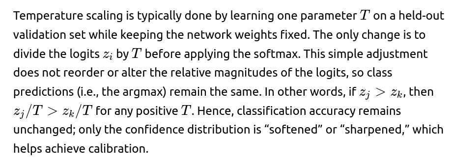
However, if T is excessively large, probabilities might become too uniform and uninformative. If T is very small, probabilities become more peaked. The best approach is to use a grid search or iterative methods on a validation set to find the T that minimizes a calibration metric (e.g., ECE). This method is widely used in modern deep learning frameworks due to its simplicity and effectiveness.

Can you combine ensembling with calibration?

Yes. Combining multiple classifiers (or multiple neural network snapshots via an ensemble) can improve both accuracy and calibration. Ensemble methods average the predicted probabilities across multiple models. Because each model might over- or under-estimate probabilities in different regions, the ensemble average often provides a naturally smoother probability estimate that tends to be better calibrated. One can then apply further calibration methods (e.g., temperature scaling or Platt scaling) on top of the ensemble’s probabilities to refine any residual miscalibration. In practice, ensembles are often among the strongest techniques for achieving both high accuracy and better calibration, but they come with additional computational cost.

---

Below are additional follow-up questions

How do you handle calibrating a model on an imbalanced dataset, and why can this be tricky?

Dealing with imbalanced data is a challenge for calibration because the model’s predicted probabilities can be dominated by the majority class, making it harder to properly estimate probabilities in the minority class range. One subtlety is that typical calibration methods (like Platt scaling or isotonic regression) often rely on having a representative set of positive and negative examples in each probability bin. If the minority class is too rare, the bins that matter most for that class might have very few examples, risking noisy or overfitted calibration mappings.

A common mitigation technique is to use a validation set specifically stratified to ensure adequate coverage of minority examples. Another approach might be to use sampling or weighting in the calibration process. For instance, you can upsample the minority class or apply class weights when fitting the calibration function so that the model’s probabilities are better tuned in the minority’s probability range. However, rebalancing can distort the overall distribution if not handled carefully, so checking the final calibrated probabilities on the true distribution is important.

How does calibration differ from discrimination (for example, as measured by AUC), and why might a model with a good AUC still need calibration?

Discrimination focuses on how well a model separates positives from negatives. For binary classification, the Area Under the ROC Curve (AUC) tells us how well the model ranks positive instances higher than negative ones. However, a good AUC does not necessarily imply correct probability estimates. A model can rank positives correctly but still produce miscalibrated confidence scores (e.g., it might assign extremely high scores even when the true likelihood is more moderate).

Calibration, in contrast, is about the agreement between predicted probabilities and observed outcomes. You can have a strong rank-ordering of examples (leading to a good AUC) but still have probabilities that do not match reality. For example, a model may consistently predict around 0.9 for positives, when in truth the actual fraction of positives at that level is only 0.7. Therefore, it might be an excellent discriminator but overconfident. If precise probability estimates are needed for decision-making (such as threshold selection, risk assessment, or resource allocation), calibration must be explicitly addressed.

How does label smoothing differ from calibration, and do they achieve the same effect?

Label smoothing is a technique often used during model training (particularly in neural networks) where instead of using hard one-hot labels, the targets are “softened” by assigning a small portion of probability mass to incorrect classes. The main goal is to prevent the model from becoming overly confident and to encourage better generalization by avoiding fitting training data too rigidly.

Calibration, on the other hand, is generally a post-training adjustment (though some methods can be integrated into training) intended to align predicted probabilities with true outcome frequencies. While label smoothing may indirectly help reduce overconfidence, it is not guaranteed to produce well-calibrated probabilities. A model trained with label smoothing can still be miscalibrated, perhaps in a different manner. Consequently, even if you apply label smoothing, it is still prudent to check calibration on a validation set and consider applying explicit calibration methods if needed.

Does post-hoc calibration guarantee a better Brier Score or log-likelihood?

Post-hoc calibration can improve the alignment between predicted probabilities and observed outcomes, which often improves scoring metrics like the Brier Score or the negative log-likelihood (both are sensitive to probability estimates). However, improvement is not guaranteed in every case. If the calibration set is small or unrepresentative, the learned calibration map might overfit or distort the probabilities in ways that hurt these metrics on unseen data.

Another subtlety is that certain calibration methods might push the probabilities toward more moderate values. If the original model was extremely confident but correct much of the time (albeit not perfectly calibrated), forcing probabilities to become less extreme might increase the Brier Score or degrade log-likelihood in some narrow scenarios. Typically, though, one can expect a well-chosen calibration approach to at least not harm, and more often to improve, these probabilistic scoring metrics when tested on data similar to the calibration set.

Could using multiple calibration techniques in combination yield better results than a single technique?

In principle, one might try combining different calibration methods by, for example, blending or stacking. For instance, you could apply temperature scaling to the logits and then feed those probabilities into isotonic regression. However, chaining multiple calibration layers can lead to overfitting, especially if the validation set is not large enough to support multiple transformations.

Moreover, certain calibration steps (e.g., isotonic regression) can already shape the probability mapping in a fairly flexible way. Adding an additional layer may not bring much benefit and could introduce complexity without clear gains. In practice, it is typically more effective to choose one robust calibration approach that suits the data size and distribution, evaluate it carefully (possibly with cross-validation), and use the simplest method that provides adequate calibration.

If different models have varying calibration levels, how do you decide which to put into production?

First, you need to clarify your objective. If the ultimate goal is purely classification accuracy or F1 score, and you do not rely on the explicit probability values, then a slightly miscalibrated model with higher accuracy might be preferable. If your application heavily depends on making threshold-based or cost-sensitive decisions (e.g., in finance or healthcare), you might place more value on well-calibrated outputs. In such settings, a model with slightly lower accuracy but significantly better calibration could be more valuable overall.

Additionally, you can combine the best-performing model’s predictions with a calibration step. If a high-accuracy model is miscalibrated, you may apply a calibration method to improve its probability estimates. Production decisions often involve trade-offs: you weigh the computational complexity of calibration, the time to implement and maintain, and the performance benefits. A thorough offline evaluation with metrics such as ECE, Brier Score, or log-likelihood—alongside standard accuracy or AUC—helps guide the best choice.

How can domain shifts or distribution changes impact calibration, and how do you mitigate such issues?

Calibration mappings learned on one distribution typically assume that new data follows the same distribution. If there is domain shift—where the test data distribution deviates from what was observed during training and calibration—previously learned calibration functions may no longer hold. For instance, if the prevalence of a class changes significantly, or if certain features have shifted, the probabilities might drift from their calibrated relationships.

Mitigation strategies include:

• Continuous recalibration: Periodically re-collect data from the new distribution and update calibration parameters.

• Online calibration: In streaming or online settings, maintain a small window or weighting scheme for recent data to recalibrate on the fly.

• Domain adaptation: Use techniques that can detect and adjust for changes in feature distributions.

• Robust calibration: If feasible, develop a calibration approach that incorporates uncertainty and does not overfit to a specific domain.

Are there more advanced or alternative calibration methods besides Platt scaling, isotonic regression, and temperature scaling?

Yes. Some examples include:

• Beta calibration: An extension of Platt scaling using the Beta distribution. It can capture skewed miscalibration patterns.

• Bayesian calibration approaches: Incorporate uncertainty about the calibration parameters, potentially providing more robust estimates, especially when data is limited.

• Spline-based or other flexible parametric methods: Fit smooth functions to the uncalibrated scores, providing more flexibility than a logistic function but less step-wise shape than isotonic regression.

Choice among these can depend on data size, distribution shape, and the complexity of miscalibration.

How can you effectively calibrate when you have extremely limited validation data?

When validation data is scarce, any calibration approach can be prone to overfitting. Parametric methods like Platt scaling or temperature scaling, which have only a few parameters, may be safer because they are less likely to overfit compared to more flexible methods like isotonic regression. Cross-validation can help mitigate the risk of overfitting: you can train your main model on part of the data, then learn calibration parameters on another fold, and finally average or choose the best parameter set.

Additionally, Bayesian calibration approaches might help quantify the uncertainty in the calibration function. Careful data augmentation could be considered, but only if you can preserve the real distribution of probabilities in the synthetic data—this is often non-trivial and domain specific.

What if your model scores come from a distribution that differs significantly from what typical calibration approaches assume? Can you still calibrate effectively?

Some classical calibration methods, like Platt scaling, assume that the uncalibrated scores can be transformed via a logistic or similar function. If these assumptions are severely violated (for example, if your scores are extremely skewed or multi-modal), the calibration might struggle. Non-parametric methods such as isotonic regression or more advanced flexible approaches (splines, Beta calibration) might handle unusual score distributions better, as they do not presume a single functional form for the mapping.

In extreme cases, you may need to transform your scores (e.g., applying a monotonic transformation that normalizes or compresses them) before applying standard calibration. Ultimately, one must empirically verify whether a chosen method is successfully producing well-calibrated results on a validation set representative of the real distribution.

In which scenarios could post-hoc calibration reduce the interpretability of the final model?

Occasionally, introducing a non-parametric or multi-parameter calibration layer can make it harder to directly interpret the raw logits of your model. For instance, isotonic regression may produce piecewise constant functions that are not straightforward to reason about. Moreover, if the main model was built with interpretability in mind (e.g., a linear model where each coefficient has a meaning in the domain), applying a separate layer that warps probabilities can obscure that transparency.

However, in many settings, interpretability focuses on local explanations for predictions (e.g., feature attributions) rather than on the calibration function itself. If the main interest is in explaining how a prediction was formed from input features, an added calibration layer typically does not obscure the main model’s logic. But the mapping from raw model scores to final probability can become less transparent, depending on the calibration method.

How should you calibrate a multi-label classifier where each sample can have multiple active labels?

In multi-label classification, each instance can be associated with multiple classes simultaneously, and you receive a probability score per label. A straightforward approach is to calibrate each label as if it were a separate binary classification task. For each label, you gather all instances, consider whether that label is active or not, and then apply a binary calibration procedure (e.g., Platt scaling or isotonic regression).

Potential pitfalls include label correlations. If certain labels tend to co-occur often (or rarely), a per-label calibration might ignore those dependencies. In practice, many teams still calibrate each label independently, as it is simpler and often effective, but they remain aware that ignoring label dependencies can introduce miscalibrations if the data has strong label correlations.

What are the pros and cons of parametric vs. non-parametric calibration approaches in large-scale scenarios?

Parametric methods (e.g., Platt scaling, temperature scaling):

• Pros:

  • Less risk of overfitting with limited data.

  • Simple to implement and fast to run, even at large scale.

  • Typically stable, requiring only a few parameters.

• Cons:

  • The chosen parametric form might be too restrictive if the model’s miscalibration pattern is more complex.

Non-parametric methods (e.g., isotonic regression):

• Pros:

  • Flexible enough to handle complex shapes of miscalibration.

  • Can fit subtle patterns (like overconfidence in certain ranges and underconfidence in others).

• Cons:

  • Can overfit if the validation set is small or not representative.

  • Potentially more computationally costly for very large datasets, though efficient implementations exist.

In large-scale applications, data size can be substantial enough to support non-parametric methods, but one still needs to ensure that the complexity of the calibration method does not exceed the complexity of the miscalibration itself.

What practical steps would you take if your model has high accuracy but exhibits pronounced overconfidence?

1. Diagnostics: Plot a reliability diagram and compute ECE or other calibration metrics to quantify the degree of overconfidence.

2. Try temperature scaling: This is often the first step in deep learning contexts because it is simple, fast, and usually preserves accuracy.

3. Evaluate Platt scaling or isotonic regression: If temperature scaling alone does not fix the problem, experiment with Platt scaling (logistic calibration). If you have enough validation data, isotonic regression might correct more nuanced patterns.

4. Retrain with a regularizing approach: As a more fundamental fix, you can incorporate techniques like label smoothing or focal loss (in classification) to reduce overconfidence at training time.

5. Check impact on business metrics: Validate that any improvements in calibration do not critically harm the overall decision-making objectives (for instance, maintaining certain recall levels or other constraints).

Do we use a separate temperature for each class in multi-class temperature scaling, or a single temperature for all classes?

In the simplest and most common form of temperature scaling for multi-class models, one scalar temperature T is learned and applied uniformly to all logits. This approach is appealing because it preserves the ordering across logits for each sample. Multi-class extensions can allow different temperatures per class, but that increases the number of parameters and complicates the method. If data is abundant and the miscalibration patterns differ significantly across classes, a per-class temperature approach could be explored. However, a single temperature is generally sufficient in many neural network scenarios and poses less overfitting risk.

If a Bayesian neural network or ensemble is already modeling uncertainty, do we still need calibration?

Even Bayesian neural networks, which produce predictive distributions, can be miscalibrated. While Bayesian methods often yield more realistic uncertainty estimates than deterministic networks, they do not inherently guarantee perfect calibration. A well-tuned Bayesian approach might require less aggressive post-hoc calibration, but verifying calibration empirically remains important.

Similarly, model ensembles tend to improve calibration compared to single models because averaging probabilities can “smooth out” extreme confidences. Nevertheless, the ensemble may still be miscalibrated in certain ranges, so a final calibration step is sometimes applied to the ensemble’s averaged scores for mission-critical tasks.

Can you perform calibration for continuous predictions in regression tasks?

Strictly speaking, “calibration” typically refers to classification probabilities. However, there is a closely related concept for regression tasks called “probabilistic calibration” or “uncertainty calibration” if the model outputs a distribution over the target variable. For instance, if a model outputs a normal distribution for a predicted variable, you can check how frequently the true values fall within certain prediction intervals. If the intervals match the expected coverage (e.g., a 90% prediction interval contains the true value around 90% of the time), the model can be considered well-calibrated in the regression sense. Methods like conformal prediction, quantile regression, or other distribution-fitting techniques can be used to ensure that the predicted distributions match reality.

Which calibration methods are commonly used for random forest predictions?

For random forests, a typical approach is to take the proportion of trees voting for the positive class as the raw predicted probability. However, these proportions are not always well-calibrated. Platt scaling (fitting a logistic regression on these proportions) or isotonic regression (applied to the predicted probabilities from the forest) are common post-processing steps. If the random forest is large and the validation set is sufficient, isotonic regression can capture more nuanced miscalibrations. If data is limited or you prefer fewer parameters, Platt scaling or temperature scaling (with a logistic link on the forest’s log-odds) may suffice.

How is a reliability diagram different from a detection error tradeoff (DET) curve in calibration analysis?

A detection error tradeoff (DET) curve typically plots false negative rates vs. false positive rates on non-linear scales (often normal deviate scales) to highlight differences in detection performance. It’s closely related to the ROC but shown differently. A reliability diagram, in contrast, plots the empirical accuracy against predicted confidence within bins. The DET curve helps see how changes in thresholds affect false accept/reject rates, but it doesn’t directly tell you whether the predicted probabilities match the true likelihood of a positive outcome. A reliability diagram is specifically designed to analyze calibration, showing if predictions are systematically over- or under-confident.

How do you apply calibration quickly and efficiently at inference time in production systems?

Once a calibration function is learned (e.g., via Platt scaling with parameters A and B), applying it at inference is minimal overhead. For each sample’s raw score s, the calibrated probability is just the logistic function with those learned parameters:

import numpy as np

def apply_platt_scaling(s, A, B):
    return 1.0 / (1.0 + np.exp(A * s + B))

For temperature scaling on deep networks, it’s just dividing logits by TT before taking the softmax—an operation that is trivial in terms of additional computational cost:

def temperature_scale(logits, T):
    # logits is a numpy array or tensor
    return logits / T

For isotonic regression, you can store the piecewise mapping (often in a lookup table or piecewise constant intervals) and perform a fast binary search for the interval in which the score falls, then return the corresponding calibrated value. In typical production systems, these transformations are computationally light compared to the main model inference. The main consideration is to ensure the mapping is well-documented and consistently applied, especially if the model is served in a distributed or multi-service architecture.

Below are additional follow-up questions

How Can We Calibrate Classifiers in Situations with Non-Stationary or Evolving Data Streams?

When you have data arriving in a continuous stream and the underlying distribution evolves over time (often referred to as concept drift), calibration becomes especially challenging because:

• The calibration mapping learned on historical data might no longer apply to future data.

• Real-time recalibration may be required if the distribution shift is significant.

A practical approach is to maintain a sliding window or incremental calibration scheme:

• Continuously monitor calibration metrics like the Brier score or Expected Calibration Error (ECE) over the most recent data window.

• If performance degrades beyond a threshold, retrain or update your calibration model using the new window of data.

• Combine techniques like online isotonic regression or incremental versions of Platt scaling.

Pitfalls include:

• Over-correction or oscillation: If you recalibrate too frequently with too few samples, the calibration mapping can fluctuate widely, leading to instability.

• Latent drift detection: You need a reliable drift detection method to trigger recalibration at appropriate times. Otherwise, you might miss important shifts or recalibrate too late.

How Do You Perform Calibration for Models That Output Multidimensional Continuous Distributions, Such as in Variational Autoencoders or Certain Generative Models?

Generative models, especially those parameterizing complex distributions (e.g., a Gaussian mixture with multiple dimensions), need a notion of calibration that goes beyond a single probability of a class. Instead, you want to assess how well the learned distribution matches the true data distribution. Some approaches include:

• Probability Integral Transform (PIT) Tests: For each dimension or marginal distribution, transform the samples using the cumulative distribution function (CDF) and check if they follow a uniform distribution on [0, 1]. This is a kind of “calibration check” for continuous distributions.

• Coverage Analysis for Predictive Intervals: For example, if the model provides a predictive region that is intended to capture 90% of the data, you can see if it truly contains about 90% of samples.

• Likelihood-Based Comparisons: Compare the model’s log-likelihood on a validation set to theoretical bounds or to a well-calibrated reference model.

Pitfalls:

• High Dimensionality: As the number of output dimensions grows, ensuring calibration across all dimensions consistently is complex.

• Model Misspecification: If the architecture or distribution family cannot represent the underlying data generation process, no calibration technique can fully correct for this mismatch.

What Are the Differences Between Label Smoothing and Temperature Scaling in Terms of Calibration?

Label smoothing modifies the training objective by distributing a small portion of probability mass to incorrect classes, making the model less confident in its predictions. Temperature scaling adjusts the final model logits post-training to reduce overconfidence. Key points:

• Label Smoothing:

  • Encourages a slightly softer distribution for each training instance.

  • Can improve generalization and reduce overconfidence.

  • Might affect the internal representation learned by the model since it changes the loss landscape.

• Temperature Scaling:

  • Keeps the original training process intact.

  • Only adds a single scalar parameter T that rescales logits before softmax on a validation set.

  • Mainly addresses the overconfidence problem without changing how the model discriminates classes.

Pitfalls:

• Underconfidence: Excessive label smoothing can make probabilities too “flat,” potentially hurting discriminative power.

• Sensitivity to Hyperparameters: The smoothing factor in label smoothing and the temperature T in temperature scaling both require tuning on a validation set.

How Do We Calibrate a Model When the Training Set Is Extremely Imbalanced, Such as 1:10,000 Ratio?

When the positive class is exceedingly rare, calibration can be very sensitive to small errors in estimating the positive class probability. Potential solutions:

• Stratified or Custom Binning: Normal calibration curves that use uniform binning might place almost all samples in near-zero bins. Using stratified binning can ensure each bin has enough positive cases to estimate observed frequency more reliably.

• Weighted ECE or Weighted Calibration Metrics: Consider weighting each instance inversely by class frequency so that positive cases have higher influence.

• Oversampling or Synthetic Data Generation: SMOTE-like methods can create synthetic minority examples to help the model learn more robust probability estimates. However, these methods require caution to avoid spurious data points.

• Separate Post-Processing for Rare Class: Some practitioners specifically train a second “rare event calibration” model on top of the main classifier’s output, focusing on the minority class distribution.

Pitfalls:

• Overfitting in Rare Class Regions: A small set of positive examples can lead isotonic or Platt scaling to overfit, especially if the partition used for calibration is too small.

• Threshold Selection vs. True Calibration: In high-imbalance scenarios, the threshold choice often matters more than the absolute correctness of the probability. If the business goal is to detect rare positives at all costs, perfect probability calibration might be secondary.

Can Multiple Calibration Methods Be Combined, and Would That Improve Results?

You could, in principle, chain or blend different calibration strategies (e.g., applying temperature scaling first and then isotonic regression), but in practice:

• Overfitting Risk: Each layer of calibration attempts to fit residual miscalibration. Adding more layers can quickly overfit if the validation set is not large enough.

• Increased Complexity: Maintaining multiple calibration transformations complicates the deployment pipeline, especially if you need real-time predictions.

• Minimal Gains: If one method already effectively corrects the major sources of miscalibration, additional methods might yield minimal incremental benefit.

Pitfalls:

• Contradictory Corrections: Two methods might have opposite corrections (e.g., one tries to increase probabilities, another tries to decrease them).

• Interpretability: A single, simple calibration mapping is generally easier to interpret and validate.

How Do You Calibrate a Model That Produces Multiple Outputs for Structured Prediction Tasks, Like Object Detection or Semantic Segmentation?

In structured prediction (e.g., object detection bounding boxes with class probabilities), you might have multiple probabilities and/or continuous parameters (like bounding box coordinates). Calibration can be considered separately for different aspects:

• Class Probability Calibration: For each detected object or segmented pixel, you still want the probability of the predicted class to align with the true likelihood. This can be treated like multiple independent calibration tasks (one per class).

• Uncertainty in Localization: For bounding boxes, you might want a notion of calibration for the predicted bounding box’s accuracy. That’s analogous to predicting error distributions or confidence intervals around the bounding box.

Pitfalls:

• Correlations Among Outputs: In object detection, probabilities and bounding box coordinates might be correlated (e.g., the bounding box confidence depends on the object class). Calibration for one dimension might not straightforwardly transfer to others.

• Computational Overhead: Calibrating thousands of predictions in a single image at inference time can be computationally expensive if not optimized.

How Could You Calibrate a Model in an Adversarial Environment Where Inputs May Be Perturbed?

In adversarial settings, attackers might craft inputs that exploit the model’s calibration gaps. For example, an overconfident region of the input space might be specifically targeted:

• Adversarial Training with Calibration Objectives: Incorporate adversarial examples into the training set and ensure the model’s probability estimates remain consistent under perturbation.

• Robust Post-Processing: Some research explores defenses that smooth the output distribution or clamp probabilities in uncertain regions. This can be viewed as a calibration step aimed at preventing extreme overconfidence on adversarial examples.

• Certifiable Bounds: Some methods attempt to provide a certified radius around each input within which predictions—and therefore calibrated probabilities—do not drastically change.

Pitfalls:

• Trade-Off Between Robustness and Calibration: Making a model robust to adversarial attacks can degrade its calibration on clean data if done improperly.

• Complex Threat Models: Different adversarial attack strategies might exploit different vulnerabilities, so calibration alone is not a universal defense.

How Would You Apply Calibration Techniques to Models That Produce Rankings Rather Than Probabilities, Such as Recommender Systems?

Many recommender systems output a ranking (or a score that is not explicitly a probability) for potential items. To calibrate these scores:

• Convert Scores to Probabilities: If the model’s ranking metric is correlated with the likelihood of user clicks, you can map the raw scores to probabilities of a user action (e.g., logistic transformation).

• Post-Hoc Calibration: Once you have a probability-like measure for an event (e.g., user-click), use Platt scaling or isotonic regression on a validation set where you know the actual click behavior.

• Segment-by-Segment Calibration: Recommender systems often face user-level or item-level heterogeneity. You may need to calibrate per user segment or item category.

Pitfalls:

• Non-Stationary User Preferences: User interests evolve, requiring continuous recalibration.

• Skew in Feedback Data: Feedback loops can lead to missing labels for items not shown to users, complicating the calibration process.

How Do We Ensure That Calibration Does Not Compromise the Model’s Overall Predictive or Classification Performance?

One of the main concerns is whether calibration can reduce AUC, F1-score, or other ranking-based metrics. Generally:

• Post-Processing Means No Change in Ranking: If you calibrate by applying a monotonic function (like isotonic regression or Platt scaling) to the scores, the relative order of predictions should remain the same. This implies the AUC and rank-based metrics are typically unaffected.

• Trade-off with Log-Loss or Brier Score: Calibration often improves log-loss or Brier score but does not necessarily harm discriminative performance. If it does, you might have an overfitted calibration model or a mismatch in data.

Pitfalls:

• Overfitting in the Calibration Stage: Overly flexible calibration (isotonic with limited data) might degrade performance on a test set. Always check on a separate hold-out set.

• Non-Monotonic Mappings: In rare custom calibration approaches that are not monotonic, the ranking could be altered.

What Are the Challenges of Using Bayesian Methods for Calibration?

A Bayesian approach might provide a posterior distribution for each parameter of the model. The hope is that well-specified priors and enough data lead to intrinsically calibrated predictive distributions. Challenges include:

• Computational Complexity: Fully Bayesian neural networks can be very expensive to train and scale.

• Model Misspecification: If the prior or likelihood is misspecified, the posterior can still be miscalibrated.

• Approximate Inference: Variational inference or MCMC approximations might not capture the true posterior accurately, leading to miscalibrated confidence intervals.

Pitfalls:

• Overconfidence in Certain Regions: Even Bayesian models can be overconfident if the approximations or priors are inadequate.

• Difficulties in Maintaining Real-Time Performance: For large-scale production, the overhead of Bayesian inference might be infeasible.

How Can We Calibrate a Model That Is Trained to Optimize a Different Objective, Such as Maximum Coverage at a Fixed False Positive Rate?

Some tasks optimize a custom objective, for example, maximizing coverage (recall) at a strict false positive rate. This can yield a model with unusual probability distributions. You can still calibrate probabilities by:

• Treating the Model Outputs as Scores: Map these scores to probabilities via Platt scaling or isotonic regression on a validation set that includes the desired coverage/fpr conditions.

• Dual-Objective Fine-Tuning: Fine-tune the model so that it meets the coverage/fpr constraint but also tries to maintain a correct probability mapping. This might be tricky to balance in practice.

Pitfalls:

• Non-Monotonic Relationship with Probability: The threshold used for coverage/fpr might conflict with a straightforward probability scale.

• Shifting Operational Points: If the false positive rate constraint changes over time, the calibration mapping might need to be updated as well.

How Do We Interpret Calibration Plots When We Have Very Few Samples in Some Probability Bins?

This is a classic problem in calibration diagnostics. When the model rarely produces certain probabilities, the bins for those probabilities might have very few samples, leading to high variance in the observed frequencies. Techniques to mitigate:

• Adaptive Binning: Instead of uniform binning, use quantile binning so each bin has roughly the same number of samples. This ensures each bin estimate has enough statistical support.

• Smoothing Techniques: You can apply kernel smoothing or lower-variance estimators in the reliability diagram computation.

• Confidence Intervals: Show error bars around each bin’s point estimate to reflect uncertainty due to small sample sizes.

Pitfalls:

• Illusory Overconfidence or Underconfidence: A small-sample bin might produce a misleading calibration curve.

• Misinterpretation of ECE: The standard ECE formula can be heavily influenced by bins with very few samples.

How Can We Approach Calibration in Semi-Supervised or Weakly Labeled Settings?

In semi-supervised learning or settings with partial/noisy labels, calibration is difficult because you do not have reliable ground truth for all samples. Possible approaches:

• Label Densification or Correction: Use techniques like self-training or consistency regularization to refine or filter out noisy labels, then calibrate using the “cleaned” set.

• Confidence-Based Self-Calibration: In some research contexts, the model’s own predictive confidence (with additional assumptions) can be used to iteratively improve calibration. This is riskier, as it can reinforce model biases.

• Leveraging Smaller, Fully Labeled Subsets: Perform standard calibration on the subset of data with reliable labels. This might still not perfectly generalize to the unlabeled data distribution.

Pitfalls:

• Biased Subset: The small labeled dataset may not reflect the overall data distribution, leading to miscalibration on the unlabeled portion.

• Circular Reasoning: Using the model’s own predictions as “pseudo-labels” can further entrench miscalibration if the model is already biased.

How Would You Perform Calibration at Different Time Horizons for Forecasting Models?

For forecasting scenarios (e.g., predicting probabilities of events over time frames like 1 day ahead, 1 week ahead, 1 month ahead), the calibration can differ across these horizons. Steps might include:

• Separate Calibration Per Horizon: If your model outputs multi-horizon forecasts, calibrate each horizon’s probabilities separately on validation data for that specific time lag.

• Time-Dependent Binning: Construct reliability diagrams or calibration curves specifically for each forecast horizon. Patterns of overconfidence can vary at different lead times.

• Contextual Features: Some calibration mapping might depend on covariates like seasonality or macroeconomic indicators. You could train a conditional calibration model.

Pitfalls:

• Data Scarcity for Longer Horizons: Farther-out forecasts might have fewer reliable observations, making calibration uncertain.

• Shifts in Dynamics: If the underlying process changes over time (e.g., new external factors), the calibration for one horizon might not hold at a later stage.

How Do We Handle the Fact That Some Models (e.g., Decision Trees, Random Forests) Produce Internal Probability Estimates That Are Already "Calibrated" by Default?

Tree-based methods in frameworks like scikit-learn often produce probability estimates by looking at the proportion of positive samples in leaves. While this can be reasonably calibrated in some cases, it’s not guaranteed:

• Check Empirically: Use a reliability diagram or ECE to confirm whether the random forest or gradient boosting probabilities are indeed well-calibrated.

• Apply Minor Post-Processing If Needed: Sometimes, a simple temperature scaling or Platt scaling can correct small biases.

• Splitting Criteria vs. Probability Estimation: Even if a decision tree is pure in certain leaves, it may overfit or have too few samples in certain partitions, leading to high variance in probability estimates.

Pitfalls:

• Overconfident Leaves: A leaf with only a handful of samples might produce a 100% positive class proportion, indicating a probability of 1.0. This can be extremely overconfident.

• Ensembles With Different Calibration Needs: Each tree in an ensemble might have different calibration biases that average out or not, depending on how the ensemble is aggregated.

Could There Be a Conflict Between Interpretability and Calibration?

Sometimes calibrating a model might add a layer of complexity that affects how easily end-users or domain experts interpret the final output:

• Added Post-Processing Step: If an interpretable model (like logistic regression) is followed by isotonic regression, the final probability is no longer just a simple logistic function of inputs.

• Model Transparency vs. Probability Accuracy: Highly interpretable models might have simpler structures that are easier to explain, but they might be less calibrated unless you specifically refine them.

Pitfalls:

• Regulatory Environments: In certain domains (like finance or healthcare), regulations require model interpretability. Post-hoc transformations might complicate compliance if not documented clearly.

• User Trust Issues: If the end-users trust a direct model output more than a post-processed one, you might need thorough explanation of what calibration is doing.

How Would You Do an Online Evaluation of Calibration If You Only Have Access to Aggregate Outcomes (e.g., overall conversion rate) Rather Than Individual Labels?

Some advertising or finance scenarios only track overall outcomes without individual instance labels. For instance, you know total conversions but not which specific user converted. Calibration is tricky here because you cannot directly compute the fraction of positives within a bin. You might:

• Experimentation Framework: Randomly bucket traffic or apply bandit-like strategies to compare predicted probabilities with actual outcomes over time.

• Aggregate-Level Constraints: If the predicted probabilities sum to a certain expected outcome, compare that sum to the observed outcomes over the same time period. This is a coarse calibration check.

• Partial Label Observability: Seek partial feedback (like post-click conversions for a subset of users) and calibrate using that subset.

Pitfalls:

• Inability to Pinpoint Miscalibration in Specific Probability Ranges: Aggregate data may mask significant miscalibration in certain bins.

• Delayed Feedback or Attribution Issues: If conversions happen days later, the real-time calibration might lag behind actual user actions.

How Can We Integrate Domain Knowledge into the Calibration Process?

If domain experts provide insights on typical frequencies or known biases, you can incorporate this into calibration by:

• Prior Adjustment: If you have a prior belief about the base rates (e.g., disease prevalence), you can incorporate that into Platt scaling or isotonic regression by weighting the samples or adjusting the intercept.

• Constraint-Based Calibration: Impose monotonic constraints or certain expected relationships (e.g., probability for event A should always be higher than event B under certain conditions).

• Expert-Labeled Subset: Use a small but expert-labeled subset with extremely accurate labels for calibration. This can anchor the probabilities in a reliable ground truth region.

Pitfalls:

• Unquantified Bias in Domain Knowledge: Experts might unintentionally provide inaccurate estimates, skewing the calibration mapping.

• Complex Domain Interactions: Real-world phenomena can have multiple confounding factors, making it hard to incorporate domain knowledge in a straightforward way.