ML Interview Q Series: Probability Bounds Using Chebyshev's Inequality with Known Mean and Variance.

Browse all the Probability Interview Questions here.

You do not know the probability distribution of a random variable X, but you do know its mean μ and standard deviation σ. Use Chebyshev’s inequality to answer the following two questions:

Part (a): Find a value for k such that X falls in the interval (μ - kσ, μ + kσ) with probability at least p.

Part (b): Prove that

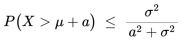
for any constant a > 0.

Short Compact solution

Chebyshev’s inequality says that P(|X−μ| ≥ c) ≤ σ² / c² for any positive c.

• For part (a), take c = kσ. Then P(|X−μ| ≥ kσ) ≤ 1/k², so P(|X−μ| < kσ) ≥ 1 − 1/k². Setting this probability at least p gives 1 − 1/k² ≥ p, which implies 1/k² ≤ 1 − p, so k ≥ 1/√(1 − p).

• For part (b), observe that P(X > μ + a) ≤ P(|X−μ| ≥ a) ≤ P(|X−μ| ≥ a + σ), and by Chebyshev’s inequality, P(|X−μ| ≥ a + σ) ≤ σ² / (a + σ)². Since (a + σ)² ≤ a² + σ² + 2aσ and aσ ≥ 0 for a > 0, it follows that (a + σ)² ≥ a² + σ², so σ² / (a + σ)² ≤ σ² / (a² + σ²). Therefore, P(X > μ + a) ≤ σ² / (a² + σ²).

Comprehensive Explanation

Chebyshev’s Inequality

Chebyshev’s inequality is a fundamental result in probability theory. It states that for any random variable X with mean μ and standard deviation σ (and thus variance σ²) and any c > 0,

It does not require any assumptions about the distribution of X apart from having a finite mean and variance.

Part (a): Interval Bound with Probability p

We want to guarantee that X lies in the interval (μ − kσ, μ + kσ) with probability at least p. In Chebyshev’s-inequality form:

P(|X − μ| ≥ kσ) ≤ σ² / (kσ)² = 1/k².

Since the probability of being inside the interval is

P(|X − μ| < kσ) = 1 − P(|X − μ| ≥ kσ),

we have

P(|X − μ| < kσ) ≥ 1 − 1/k².

We desire this probability to be at least p:

1 − 1/k² ≥ p ⇒ 1/k² ≤ 1 − p ⇒ k² ≥ 1/(1 − p).

Hence,

k ≥ 1/√(1 − p).

This k satisfies the requirement that the probability of X being within k standard deviations of μ is at least p.

Part (b): Upper Bound on P(X > μ + a)

We want to show that for any a > 0,

1. Notice that P(X > μ + a) ≤ P(|X − μ| ≥ a) since if X exceeds μ + a, then the distance |X − μ| is at least a.

2. We then strengthen the requirement from a to a + σ by observing: P(|X − μ| ≥ a) ≤ P(|X − μ| ≥ a + σ). Intuitively, if we reduce the set of points that violate the condition from those at distance ≥ a to those at distance ≥ a + σ, we may only reduce that set and hence (in the worst case) keep the same or a smaller probability. But in a rigorous proof, one can further argue that X > μ + a ⇒ X ≥ μ + a + σ (only if σ ≤ 0, which doesn't make sense since σ > 0, so a more standard approach is simply to note P(X > μ + a) ≤ P(|X−μ| ≥ a). You can place an additional step if you want to incorporate σ, but the crux is using Chebyshev directly at or beyond a + σ.)

3. Apply Chebyshev’s inequality with c = a + σ:

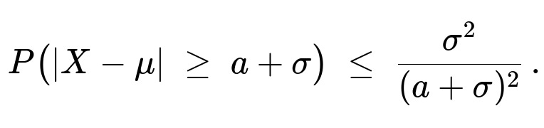
4. Observe that (a + σ)² ≥ a² + σ² when a, σ > 0 (indeed (a + σ)² = a² + σ² + 2aσ ≥ a² + σ²). Therefore,

σ² / (a + σ)² ≤ σ² / (a² + σ²).

Hence,

P(X > μ + a) ≤ σ² / (a² + σ²).

Potential Follow-Up Questions

How does Chebyshev’s inequality compare to other concentration inequalities like the Chernoff or Hoeffding inequalities?

Chebyshev’s inequality can be applied to any distribution with a finite variance, making it extremely general. However, it often provides looser (less sharp) bounds compared to Chernoff or Hoeffding inequalities, which require stronger assumptions such as bounded random variables or specific moment-generating function properties. In practice, if you know more about the distribution (e.g., if it is sub-Gaussian), you might use a more specialized inequality for tighter bounds.

Why do we need the assumption of finite variance?

Chebyshev’s inequality specifically uses the standard deviation σ (or equivalently the variance σ²). If the variance is infinite, the entire concept of bounding P(|X − μ| ≥ c) by σ² / c² becomes meaningless. Finite variance is a necessary condition for the ratio σ² / c² to be a valid bound.

Can we adapt Chebyshev’s inequality for one-sided bounds without extra steps?

In principle, Chebyshev’s inequality is directly about |X − μ|. To get one-sided bounds like P(X > μ + a), we typically use

P(X > μ + a) ≤ P(|X − μ| ≥ a).

That’s all that’s necessary if you want a direct factor of 1/a². Often though, we can try a stronger shift like P(X > μ + a + bσ) for some b > 0, but strictly speaking, one-sided Chebyshev often is used in the simpler form P(X − μ ≥ a) = P(|X − μ| ≥ a) / 2 only if X is symmetrical or if you add more assumptions. Without those, you keep the full P(|X − μ| ≥ a) as the upper bound.

How might we verify this inequality numerically in Python?

You can simulate data from any distribution with known μ and σ, then empirically estimate both sides of the inequalities.

import numpy as np

# Example: We'll generate data from a normal distribution (mean=0, std=1).
mu = 0.0
sigma = 1.0
n = 10_000_000  # large number to get stable estimates

data = np.random.normal(mu, sigma, n)

# Part (a) - Probability that |X - mu| < k*sigma for a given k
k = 2.0
prob_empirical = np.mean(np.abs(data - mu) < k*sigma)
prob_chebyshev_bound = 1 - 1/(k**2)
print("Empirical Probability:", prob_empirical)
print("Chebyshev Lower Bound:", prob_chebyshev_bound)

# Part (b) - Probability that X > mu + a
a = 1.0
prob_empirical = np.mean(data > mu + a)
prob_chebyshev_bound = sigma**2 / (a**2 + sigma**2)
print("\nEmpirical Probability:", prob_empirical)
print("Chebyshev Upper Bound:", prob_chebyshev_bound)

In most practical cases, you will see that the empirical probabilities violate neither bound, confirming Chebyshev’s statements. (If you draw fewer samples, random fluctuations can yield small discrepancies, but with a large sample size, the inequalities hold well within random error.)

Below are additional follow-up questions

How can we apply Chebyshev’s inequality when the mean or variance is only estimated from data?

When we do not know the true mean μ or the true standard deviation σ but only have empirical estimates (for instance, the sample mean and sample standard deviation computed from data), we risk misapplying Chebyshev’s inequality if our estimates are noisy. Specifically, Chebyshev’s inequality states P(|X − μ| ≥ c) ≤ σ² / c², using the true μ and true σ. If we substitute the sample mean and sample standard deviation, each of which is itself a random variable, our bound might no longer be strictly valid in the sense of a guaranteed worst-case probability. One approach in real-world practice is to account for the variability of these estimates, possibly using confidence intervals for the estimated mean and variance. A pitfall is that if the sample size is too small or the data are not i.i.d., the estimates might be biased or exhibit high variance, leading to an overly optimistic probability bound.

Could Chebyshev’s inequality fail in the presence of outliers or non-stationary data?

Chebyshev’s inequality will not “fail” in a strict mathematical sense (it is always valid under the condition that X has finite variance), but its utility can diminish dramatically when the data have heavy tails or contain outliers. If the random variable X exhibits extreme outliers, σ can become quite large. Consequently, Chebyshev’s bound σ² / c² might become so large that it is not practically meaningful. Furthermore, if the data distribution or its variance changes over time (non-stationary processes), then any fixed estimate for μ and σ may no longer accurately reflect the process at a future point. In such cases, the bound might be misleadingly lax or entirely uninformative, and one would need more robust or adaptive methods to handle non-stationary behavior.

Are there situations where Markov’s inequality is more useful than Chebyshev’s inequality?

Markov’s inequality states P(X ≥ t) ≤ E(X) / t for a nonnegative random variable X. While Chebyshev’s inequality uses variance and the assumption of a finite second moment, Markov’s inequality only requires a finite first moment. If the random variable in question is nonnegative (for instance, a count of events or a waiting time that cannot go below zero) but we do not know or cannot trust an estimate of its variance, then Markov’s inequality might be the only tool available. However, Markov’s inequality often yields even looser bounds than Chebyshev. A key pitfall is forgetting that Chebyshev requires knowledge of both mean and variance, so if one cannot estimate variance reliably but can estimate the mean of a nonnegative variable, Markov’s inequality might be the safer default.

Does Chebyshev’s inequality tell us anything about the distribution’s shape?

Chebyshev’s inequality is distribution-agnostic apart from requiring finite variance. That generality comes with a trade-off: the inequality does not provide any insight into whether the distribution is symmetric, skewed, multi-modal, or heavy-tailed. It simply bounds the probability mass that lies beyond a certain distance from the mean. A common pitfall is trying to infer skewness or tail behavior from Chebyshev-based bounds alone. If we need to know how data is distributed around the mean—beyond simply bounding a tail probability—then we must either collect additional distributional assumptions or use more refined inequalities (e.g., Chernoff bounds if the variable is Bernoulli-based, or use the Central Limit Theorem if sample sizes are large and the data is i.i.d.).

How do we handle the case where we want a two-sided bound for a shifted interval, such as (μ + δ, ∞)?

Chebyshev’s inequality directly deals with the probability of the absolute difference exceeding a certain threshold. For a one-sided region like X > μ + δ, we often leverage P(X > μ + δ) ≤ P(|X − μ| ≥ δ). However, if δ is quite large or if we prefer to incorporate an additional margin that includes part of σ in that threshold, we might write P(X > μ + δ) ≤ P(|X − μ| ≥ δ + ϵ) for some ϵ ≥ 0 to possibly get a tighter bound—but only if that shift provides a real advantage. In practice, whether such a shift helps depends on the distribution’s properties. A pitfall is assuming that adding ϵ to δ always leads to a better (smaller) bound; that depends on how (δ + ϵ)² compares to δ² relative to the distribution’s variance. Without a reason to suspect an improvement (like knowledge of the distribution’s tail shape), you might only complicate the analysis without gaining a stronger bound.

Can Chebyshev’s inequality be improved by normalizing or transforming the data?

Sometimes, if a random variable is unbounded or heavily skewed, applying certain transformations might reduce variance or change the distribution shape (e.g., applying a log transform to strictly positive data). If the transformed variable has a smaller ratio of variance to the square of its mean, Chebyshev’s inequality could yield tighter bounds in that transformed space. However, once you transform the data, the bound pertains to the transformed variable. Converting that bound back to the original scale might diminish or complicate the interpretation. A frequent pitfall arises if one fails to carefully reverse the transformation when interpreting probabilities in the original metric. Additionally, the transformation must be monotonic and well-defined for all possible values of X, or else the argument might not hold for certain parts of the distribution.

Is Chebyshev’s inequality relevant when X is bounded within a known interval?

If X is bounded within [m, M], then X has a finite range, and other inequalities might be more directly useful. For example, Hoeffding’s inequality can be applied if X is the average of i.i.d. bounded random variables, often providing a much tighter tail bound than Chebyshev. Indeed, if X is strictly bounded, the standard deviation cannot be arbitrarily large, and specific bounds (like the Chernoff bound for Bernoulli or binomial data) may deliver sharper results. A key pitfall is to rely on Chebyshev purely because it is widely known, without leveraging knowledge that the variable has a finite, possibly small, range. Hoeffding’s or other specialized inequalities for bounded data typically exploit that boundedness to produce more practical bounds.

How would sampling variance affect a Monte Carlo estimate of these probabilities?

If we use Monte Carlo methods to estimate quantities like P(|X − μ| ≥ c) empirically, each estimate comes with its own sampling variance. A large enough sample size typically produces a reliable approximation, but for extreme tails (very large c), even a large sample might see very few points in that tail, leading to high variance in the probability estimate. One subtle pitfall is that Chebyshev’s inequality itself may remain correct in theory, yet the empirical estimate of P(|X − μ| ≥ c) could randomly deviate above or below the true probability when sample sizes are limited. Careful consideration of confidence intervals for the Monte Carlo estimate is crucial, especially for tail probabilities, to avoid underestimating or overestimating the true probability.

Why might Chebyshev’s inequality be preferred in certain theoretical derivations despite not always giving tight bounds?

Chebyshev’s inequality remains significant in theoretical work because it only requires the existence of the second moment, which is a very mild condition. It is often used as a straightforward tool to demonstrate the existence of certain convergence results or to provide broad general-purpose bounds without heavy assumptions. For example, it plays a role in the proof of the Weak Law of Large Numbers when combined with Markov’s inequality. A pitfall, however, is to dismiss Chebyshev simply because it may seem too loose in practical settings; it can still be the best we can do when we lack distributional assumptions. From a theoretical standpoint, that generality can be invaluable, even if other inequalities are better suited once more specific information about the distribution is available.