
ML Interview Q Series: Probability Generating Functions for Sums of a Random Number of Dice Rolls
Browse all the Probability Interview Questions here.
You first roll a fair die once. Next you roll the die as many times as the outcome of this first roll. Let the random variable S be the sum of the outcomes of all the rolls of the die, including the first roll. What is the generating function of S? What are the expected value and standard deviation of S?
Short Compact solution
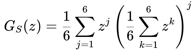
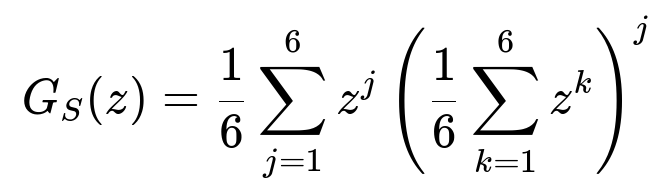
By conditioning on the outcome X of the first roll, the probability generating function of S is given by the average over X=1 to 6. Each time you get X=j, you then add j more rolls whose individual sums contribute a factor (1/6)(z + z^2 + ... + z^6). Hence,
Using the first and second derivatives of G_S(z) at z=1, the expected value of S is 15.75 and the standard deviation is approximately 7.32.
Comprehensive Explanation
The random variable S is defined by two stages of rolling a fair six-sided die. First, you roll it once and call the result X. Then, you roll the die X more times and sum up those additional rolls with the initial roll. Formally,
S = X + X1 + X2 + ... + X_X
where X is the result of the first roll, and X1, X2, ..., X_X are the results of the next X rolls.
The probability generating function G_S(z) = E(z^S) is best handled by conditioning on X:
E(z^S) = (1/6) * Σ_{j=1 to 6} E(z^S | X = j).
Once we fix X=j, the sum S becomes j plus the sum of j i.i.d. random variables each uniformly distributed over {1,2,3,4,5,6}. Denote these i.i.d. variables by X1,...,Xj. Therefore,
S = j + (X1 + X2 + ... + Xj).
Hence,
E(z^S | X = j) = E(z^(j + X1 + ... + Xj)) = z^j * E(z^(X1 + ... + Xj)).
Each Xn for n=1 to j has generating function (1/6)(z + z^2 + z^3 + z^4 + z^5 + z^6). Since they are independent,
E(z^(X1 + ... + Xj)) = [(1/6)(z + z^2 + z^3 + z^4 + z^5 + z^6)]^j.
Putting it all together,
G_S(z) = (1/6) Σ_{j=1 to 6} z^j [ (1/6) (z + z^2 + z^3 + z^4 + z^5 + z^6) ]^j.
This directly yields:
To find E(S), you take the first derivative of G_S(z) and evaluate at z=1. For the variance or standard deviation, you use the second derivative of G_S(z) at z=1 and apply Var(S) = E(S^2) – [E(S)]^2. The compact calculation yields:
E(S) = 15.75 E(S^2) = 301.583, so Var(S) = 301.583 – (15.75)^2, and thus std(S) ≈ 7.32.
Additional Follow-up Questions
How would the generating function change if the die were not fair?
In that scenario, you would replace any uniform probabilities 1/6 with the corresponding probability p_i for i in {1,2,3,4,5,6}. Specifically, if the first roll X has probabilities p_1, p_2, ..., p_6, and each subsequent roll has probabilities q_1, q_2, ..., q_6 (possibly the same distribution as the first roll or maybe different), you would write:
G_S(z) = Σ_{j=1 to 6} p_j z^j [Σ_{k=1 to 6} q_k z^k]^j.
All other steps for deriving E(S) and Var(S) would remain analogous, but the computations would involve those probabilities p_j and q_k instead of the uniform value 1/6.
Why do we evaluate the generating function at z=1 for the mean and variance?
The probability generating function G_S(z) = E(z^S) encodes the distribution of S. By taking the derivative with respect to z and evaluating at z=1, we extract the moments of S. Specifically, d/dz of z^s (with s as a random variable) at z=1 helps isolate E(S) when we multiply by the appropriate factors. Similarly, the second derivative at z=1 helps retrieve E(S(S – 1)), from which one can compute E(S^2) and hence the variance.
Could we use a moment generating function (MGF) instead?
Yes. The moment generating function of a random variable S is M_S(t) = E(e^{tS}). For discrete random variables, the probability generating function G_S(z) = E(z^S) can be seen as a “discrete” analog of M_S(t). The approach is similar, but the expansions would replace z^k with e^{tk}. In many theoretical settings, one or the other is more convenient. For dice rolls and discrete outcomes, the probability generating function is often more direct.
Are there any edge cases to consider?
One edge case might be the scenario where X=1 occurs frequently. That still poses no conceptual difficulty, because if X=1, S is simply 1 plus one additional die roll. Another edge case is if you had a degenerate die (like always rolling the same value). That would dramatically simplify or alter the generating function. However, as long as X remains a well-defined random variable, the conditional approach works the same way, and the formulas remain valid.
Below are additional follow-up questions
How would we compute the probability that the sum S exceeds a certain threshold t?
To compute P(S > t), one straightforward approach is to rely on the probability generating function or to set up a recursive formulation for the distribution of S. However, for large t, a direct summation might be computationally expensive. One could proceed as follows:
Condition on the first roll X = j. In that case, the sum S = j + X1 + ... + Xj, where each Xi is uniform on {1,...,6}.
Compute P(S > t | X = j). This reduces to computing P(X1 + ... + Xj > t – j). We can do this by standard convolution methods for the discrete uniform distribution.
Finally, weight by P(X = j) = 1/6 and sum over all j.
A potential pitfall arises if t is very large. Then the number of additional rolls, X, could also be large with non-negligible probability, making direct combinatorial or convolution methods quite expensive. A practical workaround might be Monte Carlo simulation, drawing many samples and estimating the probability empirically. However, simulation can suffer from variance issues if t is so large that we rarely see sums exceeding t. Techniques like importance sampling or large-deviation approximations can mitigate this.
What if we want to approximate the distribution of S without explicitly using the generating function?
When the distribution or the die is more complex, computing the generating function or its derivatives might be cumbersome. One alternative is to approximate using simulation:
Generate a large number of samples of S by repeatedly (1) rolling the die for the first outcome X, (2) rolling X more times, and (3) summing those results.
Construct an empirical distribution of the sums.
Estimate the mean, variance, or any other statistic from that empirical distribution.
A subtle issue is that if the distribution is heavy-tailed (not in this simple uniform case, but could be if generalized to other distributions), you might need a large sample to get a stable estimate of the high quantiles or tail probabilities. Another potential pitfall is that naive random sampling might miss rare but influential events (for instance, rolling a 6 first and then getting several 6s in a row). Techniques like stratified sampling or importance sampling help address this.
How would we approach finding the median or other quantiles of S?
The median (the 50th percentile) or other quantiles can be found theoretically by constructing the cumulative distribution function (CDF) of S:
From the probability generating function G_S(z), in principle, one can derive the entire probability mass function (PMF) by expanding the polynomial. Summing the PMF up to the point it exceeds 0.5 gives the median.
However, the algebra might be extensive. Another approach is to use a recursive relationship or direct convolution based on the total number of rolls.
A practical method is again simulation, collecting enough samples of S and then sorting or using a selection algorithm to find the median.
A potential pitfall is that for certain discrete distributions, multiple values might hold 0.5 in the CDF. In such a case, the “median” could be ambiguous or might need to be defined as the midpoint of an interval. Also, especially with a random number of terms in the sum, the distribution can exhibit more spread than a fixed-sum scenario, so the median might not be as intuitively close to the mean.
What if we change the number of sides on the die, say to an N-sided die?
If the die is N-sided, labeled 1 through N, the analysis remains structurally the same, but you replace 6 with N. For example:
The first roll X is uniform on {1,...,N}.
The subsequent rolls (X times) each follow the same uniform distribution on {1,...,N}.
The generating function is G_S(z) = (1/N) Σ_{j=1 to N} z^j [ (1/N) (z + ... + z^N) ]^j.
The main difference is that the formulas for the mean and variance would incorporate N in place of 6, leading to:
E(S) = E(X) + E(X)*E(X1) = (N+1)/2 + (N+1)/2 * (N+1)/2, for instance, if all sides are equally likely. The same logic extends to the higher moments and standard deviation. A potential subtlety arises if N becomes very large (like 100 or 1000), which may make expansions unwieldy, and might push you toward approximation via simulation.
How can we verify that our analytical results match actual outcomes in a real experiment?
A common technique is to perform a chi-square goodness-of-fit test or a Kolmogorov–Smirnov test, comparing the observed distribution of sums from experimental or simulated data to the theoretical PMF derived from the generating function. One can:
Generate a large sample of outcomes from actual physical dice rolls or from a pseudo-random simulation.
Compute the frequencies of each observed sum.
Compare to the probabilities predicted by the theory.
Potential pitfalls include not collecting enough experimental data, which can lead to large statistical fluctuations. Dice that are not truly fair (slightly unbalanced or chipped) will systematically deviate from the theoretical distribution. For large sums, you need a bigger sample size to reliably measure tail behavior.
What if each subsequent roll depends on the first roll’s outcome in a non-uniform way?
Sometimes, you might have a scenario where the first roll’s result not only determines how many times you roll again but also changes the probability distribution for each subsequent roll. For instance, if X=6, maybe subsequent rolls are more likely to be smaller values (some contrived, weighted scenario). In that case, you would define a conditional distribution for X1,...,Xj that depends on j:
If X=j, each subsequent roll is distributed according to a specific probability distribution p(k | j).
The generating function approach still works: G_S(z) = Σ_j p(X=j) * z^j * [E(z^X1 | X=j)]^j, but now E(z^X1 | X=j) depends on j.
A pitfall is ignoring correlation structures: once you break the independence or the identical distribution assumption, you must handle each conditional distribution carefully. Large-scale expansions or direct simulation might be the more feasible route, but you have to keep track of how the distribution changes for each j.
How would the solution look if we excluded the first roll from the sum?
Sometimes the problem is posed differently: the first roll only decides how many subsequent rolls to make, but is not included in the sum. Then S would be the sum of X i.i.d. rolls, where X is the result of the first roll. In that scenario:
S = X1 + ... + X_X, without the initial X itself.
The generating function would be G_S(z) = E( [E(z^X1)]^X ).
Specifically, if X is uniform on {1,...,6} and each Xi is uniform on {1,...,6}, then G_S(z) = (1/6) Σ_{j=1 to 6} [ (1/6)(z + ... + z^6) ]^j.
A subtle real-world issue might arise if one misreads the question, inadvertently adding the first roll to the sum or forgetting to do so. This changes the mean and variance significantly, so clarity in problem setup is critical.
What if we want to test a hypothesis about the fairness of the die using the distribution of S?
In real scenarios, you might only observe the final sum S from multiple trials (each trial consists of the first roll plus the subsequent rolls). You can try to back-infer whether the die is fair. The distribution of S is quite sensitive to the underlying distribution of each face value:
You would form a likelihood function for the observed sums given a hypothesized probability distribution of the die’s faces.
By maximizing this likelihood or applying Bayesian methods, you could estimate the probabilities p_1,...,p_6.
One pitfall is identifiability: if your sample size of full trials is limited, you might not have enough resolution to distinguish slight biases in the die. Another challenge is that the first roll has the same probability distribution as subsequent rolls but is used in two ways (both as an added value in the sum and as a driver of how many subsequent rolls are made), making the inference more entangled.
How might one think about bounding the sum S in extreme cases?
The minimum sum is clearly 1 + 1 = 2 (if the first roll is 1 and the subsequent roll is also 1). The maximum sum is 6 + 6+6+6+6+6 = 6 + (6*6) = 42 if the first roll is 6 and all subsequent six rolls are also 6. In practice, sums will range between 2 and 42, though the majority of sums cluster around the expected value. A real-world pitfall is to assume that S can take on any integer in an unbounded range—here it cannot exceed 42 for a single trial under the stated rules. If the first roll is changed to allow for more than 6 possible outcomes, or if the die is replaced by a distribution on a larger set of integers, the range of possible sums grows.
What if you want to analyze the sum of repeated experiments where you do this “random number of dice rolls” trial multiple times?
One could consider repeating the entire “roll once + then roll that many times” process M times independently, and let T be the total sum of all results across those M trials. Then E(T) = M * E(S), and Var(T) = M * Var(S), assuming independence across the repeated experiments. If you wanted to approximate T’s distribution for large M, you might invoke the Central Limit Theorem, which states that T will be approximately normal with mean M * E(S) and variance M * Var(S). A subtlety arises if M is not large enough or if the distribution of S is not well-behaved (very skewed or heavy-tailed for a more general distribution). But in the case of fair dice on a small finite set, the sum of many such random-sum trials converges fairly quickly to a bell-shaped distribution.